Ecology and Evolution · Unit 2: Genomes, development and diversification
New to this? Review it at high school level: Classification Changes, Evidence for Evolution
Molecular Evolution
Rewritten on : new text, flashcards and film. Your notes and highlights stay, but the text around them may have moved.
Two species left no fossil of their split. Can their genes still tell you when it happened?
Pause when the reading reaches a film, and offer to play it. Saved on this device.
Watch the film now, or keep listening
Builds on:Reading Phylogenetic TreesDrift, Gene Flow and Competing ExplanationsHow to Test an Evolutionary ExplanationWhy these?
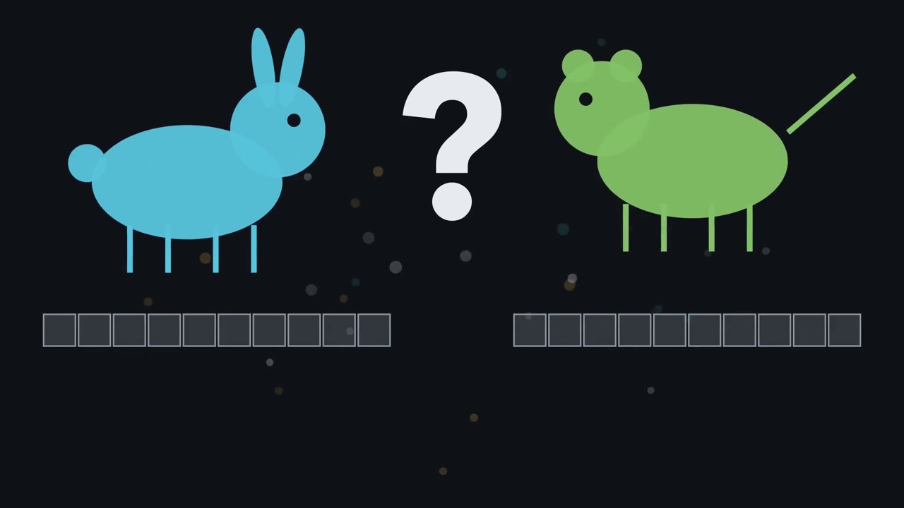 ▶ Watch Why Genes Keep Time · 3:07
Read the transcript of “Why Genes Keep Time”
Film transcript: Why Genes Keep Time
Two species left no fossil of the moment they split. Can their genes still tell you when it happened? Line up the same gene from both, and some sites differ. Start with one ancestral population. It splits into two lineages, and each keeps gaining mutations. Some spread until every member of the lineage carries them. A mutation that has spread like that is a substitution. Substitutions build up on both branches, starting from the common ancestor. So the differences you count between two species come from both branches added together. If substitutions pile up at a steady pace, their count measures time. But why should the pace be steady at all?
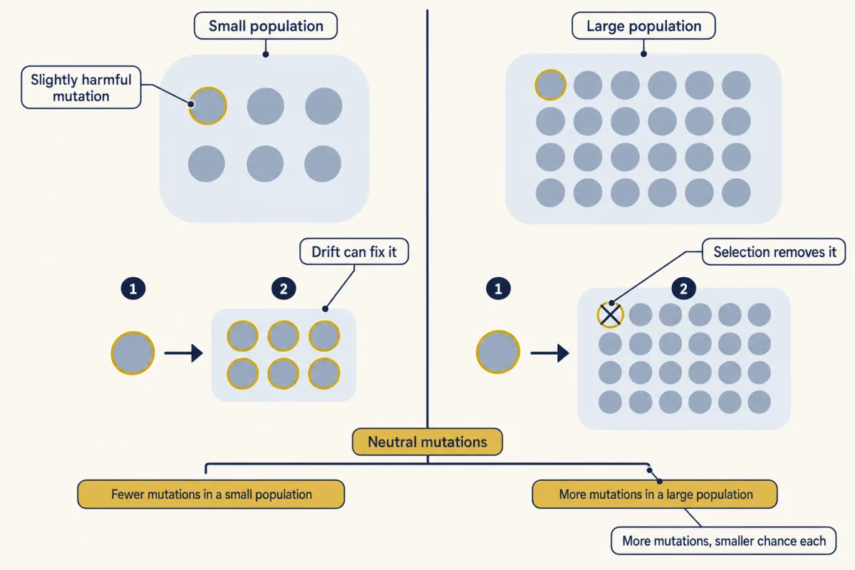
The answer lies inside a population. Picture two populations, one small and one large. Every generation, each copies the same gene. Follow only the neutral mutations. They make no difference to survival or reproduction. Suppose the large population were ten times bigger. It makes ten times more new mutations each generation. Does it pile up substitutions ten times faster?
No. Each new neutral mutation starts as one copy among many. In the large population, its chance of spreading to everyone is smaller, by the same factor. More mutations, but each one is less likely to spread. The two effects cancel. On average, neutral mutations become substitutions at the rate they arise, whatever the population size. That steady input makes the clock tick.
Now try to read a count as time. One distance could mean a fast rate over a short time. It could also mean a slow rate over a long time. The sequences alone cannot tell which. You need one date from outside the sequences. The commonest is a fossil. If two splits share a rate, one dated split can date the other. But a fossil only shows the group existed by then. The real split was earlier, by an unknown margin. So a fossil gives a minimum age. One limit already matters. The clock counts neutral changes. A mutation removed by selection never becomes a substitution, so a tightly constrained gene ticks slowly. So neutral changes pile up, on average, at the rate they arise.
Count them, add one dated split, and the count becomes time.
From the film
- A substitution is a mutation that has spread to every member of a lineage.
- Differences between two species build up on both branches since their common ancestor.
- On average, neutral mutations become substitutions at the rate they arise, whatever the population size: a bigger population makes more, but each is less likely to spread.
- Sequences alone cannot tell a fast rate over a short time from a slow rate over a long one; an outside date, usually a fossil, is needed, and it can date another split only if the two share a rate.
- The oldest fossil of a group gives a minimum age: the real split was earlier.
Genes can roughly date a split that left no fossil, and show whether selection or chance shaped what changed.
The one idea. On average, neutral changes (no effect on survival or reproduction) become substitutions at the rate they arise, whatever the population size. So neutral differences between two species pile up steadily, and one dated split turns their count into years. A departure from that neutral count is a clue to selection, not proof.
Scope: neutral sites in the same gene in both species, corrected for hidden changes; the dated split and the target must share a steady rate. Slightly harmful mutations break it: their rate depends on effective population size.
Sequences as a record
The first film counted substitutions, mutations that have reached fixation (every member of the lineage carries them), assuming you compare the same gene and see every change.
The same gene means orthologous: both copies descend from one ancestral gene, split by speciation rather than by duplication (the gene-family copies in How Signaling Evolved are mostly duplicates). Sequencing and genomes covers obtaining them. Call p the proportion of aligned sites that differ.
Predict. Two sequences differ at 30% of aligned sites (p = 0.30). Did fewer than 30 substitutions per 100 sites happen since they split, exactly 30, or more?
Check your prediction
More. A site can change twice, or change back (A to G, then G to A), hiding the first change. So p underestimates the true number of substitutions, more so as sequences diverge.
A corrected distance, D, estimates the real number of substitutions per site. The simplest correction (Jukes and Cantor) assumes all four bases replace one another at one rate; take its form as given (ln is the natural logarithm):
D = -(3/4) x ln(1 - (4/3) x p)
For p = 0.30, 1 - 0.40 = 0.60, ln 0.60 = -0.511, and D = 0.383: over a quarter more change than you see. For small p the correction is tiny: p = 0.012 gives D = 0.0121. The tree relating the sequences is itself an inference with a stated support, as in reading phylogenetic trees.
Why the clock ticks
Emile Zuckerkandl and Linus Pauling saw in the early 1960s that hemoglobin differences grew roughly in proportion to fossil-dated time since a split. The first film showed why; here is the rate.
In words New neutral mutations arise at two N mu per generation; each fixes with probability one over two N; so the substitution rate K equals the neutral mutation rate mu.
- N“N”
- diploid individuals, so 2N copies of each site
- mu“mu”
- neutral mutations per site, per copy, per generation
- K“K”
- neutral substitutions per site, per generation, in one lineage
Sanity check N = 100, mu = 10−8: 2 × 10⁻⁶ new mutations per generation × 1/200 = 10−8 = mu.
The fixation chance of one new neutral copy is 1/2N only in an ideal population (constant size, random mating); population genetics derives it. K = mu is an average; real substitutions arrive irregularly. Two steps link K to measured distance:
- Per year, the clock rate r is K divided by generation time, so at the same per-generation mutation rate, long generations mean fewer substitutions per year.
- Between two tips, D = 2rt after a time t, if both branches share the rate r.
Motoo Kimura reached the neutral theory in 1968 from the other direction, arguing that protein comparisons implied too many substitutions for selection to pay for each in selective deaths. He proposed that most substitutions are neutral or nearly neutral mutations fixed by random drift, while most strongly harmful mutations are removed before they spread. The theory does not say all mutations are neutral, or that selection is unimportant for traits.
Reading time: calibration
The molecular clock says the expected number of changes on a branch is its rate times its duration. The first film’s outside date is a calibration; besides a fossil, sequences sampled at sufficiently different known dates, such as virus samples or ancient DNA, can calibrate a tree.
Worked problem (illustrative data). Two species that fossils show split 3.0 million years ago differ by a corrected 0.012 substitutions per site in a gene. A second pair differs by 0.024 in the same gene. When did the second pair split? Assume one constant rate on all four lineages, an exact calibration date, and negligible variation in the ancestral population (see Going deeper).
- Set up the model. D = rt + rt = 2rt, with r the rate per lineage and t the time since the split.
- Calibrate. r = 0.012 / (2 x 3,000,000 years) = 2.0 x 10⁻⁹ substitutions per site per year.
- Date the target. t = 0.024 / (2 x 2.0 x 10−9) = 0.024 / (4.0 x 10⁻⁹) = 6.0 million years. Check: 2 x 2.0 x 10−9 x 6,000,000 = 0.024.
Forgetting the factor 2 in step 3 gives 0.024 / 2.0 x 10−9 = 12 million years. Since a real fossil calibration is only a minimum, both splits may be older. Try it on the line below.
- D = 2rt, through the calibration
- fossil calibration (3.0 million years)
- target distance
- date read from the line
- factor 2 forgotten (D = rt)
- 1. Calibrate: r = D / (2t)
- 2. Date the target: t = D / (2r)
- Without the factor 2: t = D / r
In this sketch: slider values other than 0.012 and 0.024 are illustrative; one constant rate on both lineages, the calibration date treated as exact, and ancestral polymorphism ignored. The fossil date is a minimum, so the dates may be older.
Distance builds up on two branches, so D = 2rt: use the factor 2 when you find the rate and again when you find the date.
When the tick rate varies
Rates differ between branches: in Drummond and colleagues’ 2006 marsupial analysis, the fastest branch of the most probable tree was estimated to evolve 2.7 times faster than the slowest. Relaxed clocks let each branch have its own rate. Bayesian dating commonly treats a fossil calibration as a range of possible ages, not a point; even with abundant data, the dates stay sensitive to the rate model and calibration ranges put in.
The mutation rate itself varies. Bergeron and colleagues in 2023 sequenced parents and offspring from 68 vertebrate species and found per-generation germline mutation rates differing 40-fold, around 10−8 per site per generation in mammals. So mu is no constant, and turning it into a per-year rate takes assumptions about neutrality and generation time.
Some mutations are not quite neutral. For these, the effective population size, Ne, matters: the size of an ideal population that drifts as strongly as the real one (the smaller Ne, the stronger drift).
Predict. A new mutation lowers fitness by 1 part in 10,000 for each copy carried. Is it more likely to become a substitution when Ne is 1,000 or 100,000?
Check your prediction
When Ne is 1,000: chance swings dwarf so small a cost, and it fixes at about 80% of the neutral rate (simple diploid model, constant Ne; other dominance or demographic assumptions shift it). At 100,000, selection wins and it almost never fixes. This is Tomoko Ohta’s 1973 nearly neutral theory: many mutations are slightly deleterious, with costs of the order of 1/Ne, and their substitution rate depends on Ne.
Reading selection in coding sequences
Where selection acts, substitutions depart from the neutral count: purifying selection can make amino-acid changes lag, and positive selection can make them run ahead. The second film shows two ways to catch that in a real gene.
Read the transcript of “Reading Selection in Genes”
Film transcript: Reading Selection in Genes
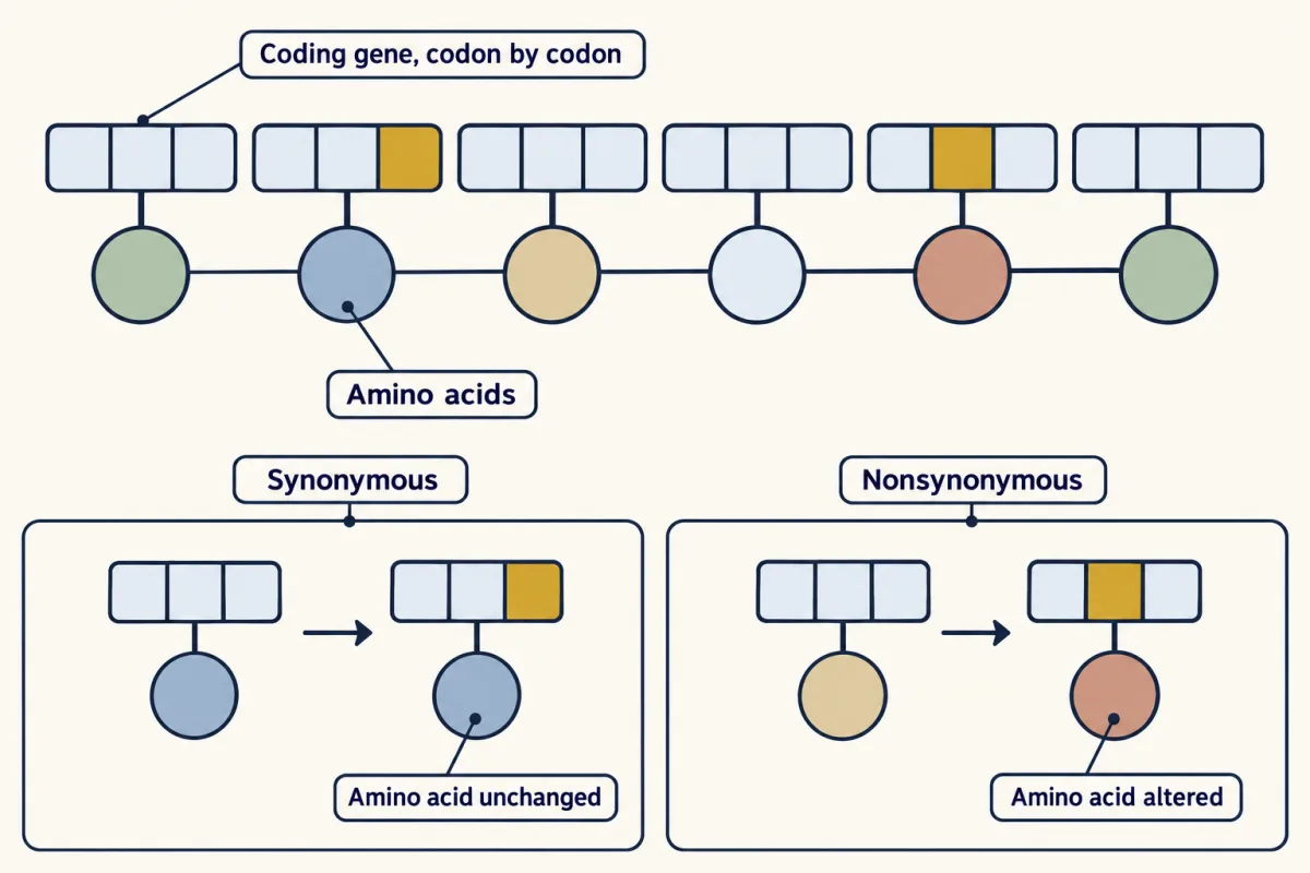
Where selection acts, changes depart from the neutral count. Purifying selection can make them lag; positive selection can make them run ahead. So how could you catch that in a real gene? Here is the trick. Find two kinds of change in the same gene that neutrality says should behave alike. If they part ways by more than chance allows, selection may be at work. Take a coding gene, read three letters at a time. The genetic code has several codons for most amino acids. So some changes keep the amino acid. These are synonymous. Other changes alter the amino acid. These are nonsynonymous, or replacement, changes. If synonymous changes are neutral, they are a built-in control for the replacements.
Count each kind along a branch, per site where it could happen. Call them dN and dS. Their ratio is called omega. Below one, replacements were fixed more slowly than silent changes. That suggests purifying selection removed some.
Near one is consistent with neutrality. Above one suggests positive selection. A second test uses variation inside a species. In 1991, John McDonald and Martin Kreitman applied it to the Adh gene of fruit flies. The gene makes alcohol dehydrogenase. Sort every change into a table. The columns are replacement and synonymous. One row holds variants within a species. The other holds differences fixed between species. Under neutrality, a variant within a species is a passing stage, on its way to fixation or loss. So both rows should hold the same ratio of replacement to synonymous changes. The variants row fills first, and it is mostly synonymous.
If replacements were neutral, what should the fixed row look like? Neutrality predicts the same ratio. Instead, the fixed row held more replacements than the variants predicted. McDonald and Kreitman suggested this reflected adaptive fixation. Here each kind of change is the control for the other. So this test needs no clock and no dated split. Both tests are model inferences, and each model can fail. A signal like this still needs further checks before it counts as adaptation.
Both tests ask the same question. Did one kind of change keep pace with the neutral count? A departure is a clue to selection, not proof.
From the film
- A synonymous change keeps the amino acid; a nonsynonymous, or replacement, change alters it.
- If synonymous changes are neutral, omega = dN/dS reads selection on the protein: below 1 suggests purifying selection, near 1 is consistent with neutrality, above 1 suggests positive selection.
- The McDonald-Kreitman test compares the ratio of replacement to synonymous changes among variants within a species with the same ratio among differences fixed between species.
- At Adh in fruit flies, fixed differences held more replacements than the variants predicted, which McDonald and Kreitman suggested reflected adaptive fixation.
- Each test is a model inference: a departure from the neutral count is a clue to selection, not proof, and needs further checks before it counts as adaptation.
Why count per site? Given the genetic code, most single-base changes in a codon alter the amino acid, so a gene offers roughly three nonsynonymous sites for every synonymous one, and raw counts would overstate amino-acid change about threefold.
Worked problem, step 4. For the second pair, a different gene has dN = 0.004 and dS = 0.040 substitutions per site. Omega = 0.004 / 0.040 = 0.10: the signature of purifying selection removing most amino-acid changes, though the gene still evolves; omega alone cannot rule out a few adaptive changes hidden in the average.
Predict. One gene has 3 codons under strong positive selection and 297 under strong constraint. Is a gene-wide omega likely to reveal the 3?
Check your prediction
Probably not. A gene-wide omega averages over all sites, so 297 constrained codons usually hold it below 1 unless the three change extremely fast. Codon models can instead estimate omega for a branch or a class of sites.
A polymorphism is a variant that still varies within a species. The second film’s Adh counts, from three Drosophila species (McDonald and Kreitman, 1991):
| Adh changes | Replacement | Synonymous | Replacement : synonymous |
|---|---|---|---|
| Fixed between species | 7 | 17 | 0.41 |
| Variable within species | 2 | 42 | 0.05 |
Is the gap chance? Replacements are 7 of 24 fixed differences (29%) but 2 of 44 polymorphisms (5%); their G-test put the chance of so large a gap, if the rows matched, at P = 0.006. The table is partly independent evidence beside omega.
When the signal misleads
Besides the power problem of gene-wide omega, each test’s model can fail:
- McDonald-Kreitman. It needs no clock but treats synonymous changes as neutral. Slightly harmful replacement variants linger as polymorphisms but rarely fix, inflating the variable row and hiding adaptation; a change in population size can mimic the signal.
- Omega within one population. The differences sampled are mostly recent polymorphisms not yet sorted by selection, so omega near 1 can arise under selection and does not establish neutrality.
- The synonymous control. In Enterobacterales, the bacterial group that includes E. coli, Rahman and colleagues (2021) found non-neutral synonymous substitutions; treating all as neutral inflated omega, and corrected values averaged 80% of standard estimates.
- Branch-site tests, which ask whether some codons changed faster on one chosen branch, assume one base changes at a time, so one mutation hitting adjacent bases looks like rapid amino-acid change. Venkat, Hahn and Thornton (2018) simulated mammal- and fly-based alignments without positive selection; such multinucleotide mutations can make the test report it.
Design problem
A branch-site test flags positive selection in an immune gene on one primate lineage. Before you believe it, what would you check?
Saved in this browser only.
One way to do it
- The data. Check the alignment around the flagged codons; confirm every sequence is a true ortholog, not a paralog (a duplicated copy) or misassembled.
- The model. Simulate alignments on the same tree with no positive selection but realistic multinucleotide mutations and base composition; if the test often fires, the result is weak. Check codon-usage bias, since selection on synonymous sites changes dS.
- A second line of evidence. Build a McDonald-Kreitman table from polymorphism within the species and fixed differences from a close relative, with an outgroup (a more distant species) to place the fixed changes on this lineage. An excess of fixed replacements adds partly independent support, under the same synonymous-neutrality assumption.
- Function. Reconstruct and express the ancestral and derived proteins, and measure the property that matters, such as binding to a pathogen protein. Even then, report a model inference supported by evidence, not an observation of adaptation.
Going deeper
The mutation-rate numbers
Bergeron and colleagues’ survey used 151 trios. The 36 mammals sampled averaged 7.97 x 10⁻⁹ mutations per site per generation, and the four classes sampled did not differ significantly overall.
Variation already in the ancestor
In a simple model (neutral autosomal genes, a randomly mating diploid ancestral population of constant size, no gene flow after the split), two species’ gene copies trace back to an ancestral copy on average about 2Ne generations older than the species split: with Ne = 10,000 and 20-year generations, about 0.4 million years, 13% of the 3-million-year calibration. So a raw gene divergence runs old. A calibrated date can err the other way: the calibrating gene split is older too, so the rate comes out too high and the second date too young (6.0 million years, where with the same offset the species split was about 6.4).
Your notes
Select any text in the lesson to highlight it or add a note to it. Your highlights and notes are saved in this browser and collected in your notebook.
This browser is not letting the site save anything (a private window or strict privacy settings), so highlights and notes will be lost when you leave the page.
How we measure it
Fossil-calibrated molecular dating
Branch lengths estimated from sequences are converted to time with external age information: a fossil that sets a minimum age for a node, or sequences sampled at known, sufficiently different dates. Bayesian relaxed-clock methods let rates vary among branches and represent calibration uncertainty as a prior distribution on node ages.
Codon-model estimation of dN/dS
Aligned coding sequences are analysed on a phylogeny with a model that separates nonsynonymous from synonymous substitutions, each counted per available site. The ratio omega = dN/dS, estimated by maximum likelihood for a gene, a branch or a class of sites, measures how amino-acid changes have fared relative to silent ones.
McDonald-Kreitman test
Changes at one locus are sorted into a two-by-two table: replacement or synonymous, and polymorphic within species or fixed between species. Under neutrality the replacement to synonymous ratio is expected to be the same in both rows; an excess of fixed replacements suggests adaptive fixation, and an excess of replacement polymorphisms suggests weakly harmful variants.
Parent-offspring trio sequencing
The genomes of two parents and their offspring are sequenced at high coverage, and sites where both parents are homozygous for the reference base and the offspring is heterozygous are taken as candidate new mutations. Correcting for the callable part of the genome and for missed mutations gives a per-generation germline mutation rate.
Practice questions on this lesson (3) → MCAT-style, original, each with an explanation
Where this lesson fits
Before thisReview first
- Reading Phylogenetic TreesThis course · Lesson 2
You need to read trees and see that branch lengths and split points are inferences before dating a split.
- Drift, Gene Flow and Competing ExplanationsThis course · Lesson 4
Fixation of neutral variants by drift, and the role of effective population size, is used here without being re-taught.
- How to Test an Evolutionary ExplanationThis course · Lesson 1
This lesson treats a departure from the neutral count as a clue to selection, not proof, which follows that testing logic.
After thisStudy next
- Evolution of DevelopmentThis course · Lesson 6
It uses sequence comparison and tests of selection on coding versus regulatory changes to ask what changed in evolution.
- Speciation: How Barriers to Gene Flow EvolveThis course · Lesson 7
Dated splits and gene divergence between species are used to ask when and how barriers to gene flow evolved.
- Human Evolutionary History: An African Origin and Archaic AncestryThis course · Lesson 9
It applies calibrated divergence dating and ancestral variation to when human populations split.
Elsewhere on the siteFilms, simulations and method films in other courses
- Fluctuation test: induced or already there?Simulation · Genetics and Molecular Biology
Mutation rate sets the neutral substitution rate here, and this fluctuation test shows mutations arise before selection.
- Why Dominance Does Not Spread an AlleleFilm · Genetics and Molecular Biology
It shows how drift and selection change allele frequencies, the basis for fixation of neutral and advantageous mutations.
- Before the Phage ArrivesFilm · Genetics and Molecular Biology
New mutations arising at a steady rate are the raw material the clock counts.
- The Molecule Behind the TreeFilm · Biology
It shows ribosomal RNA sequence differences used to infer ancestry across all cellular life.
Suggested by an AI model from the lessons themselves, then checked. How we use AI
Finish line
Test yourself
8 questions
Practice and MCAT-style, with explained answers.
Next · Lesson 6
Evolution of Development
Some lake sticklebacks have almost no pelvis, yet their Pitx1 protein is unchanged. If the protein did not break, what did?
Continue →