Ecology and Evolution · Unit 1: Evidence and evolutionary reasoning
New to this? Review it at high school level: Building a Tree of Life
Reading Phylogenetic Trees
Rewritten on : new text, flashcards and film. Your notes and highlights stay, but the text around them may have moved.
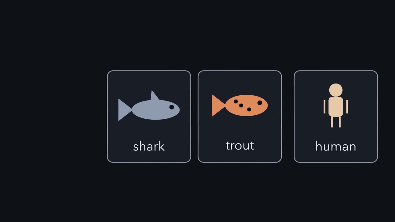
Is a trout more closely related to a shark, or to you?
Pause when the reading reaches a film, and offer to play it. Saved on this device.
Watch the film now, or keep listening
Builds on:How to Test an Evolutionary ExplanationWhy these?
 ▶ Watch Relatedness Lives at the Nodes · 3:06
Read the transcript of “Relatedness Lives at the Nodes”
Film transcript: Relatedness Lives at the Nodes
Is a trout more closely related to a shark, or to you? The two fish look alike. A tree gives a different answer. A phylogenetic tree is a hypothesis about ancestry. The living species sit at the tips. Here are five: lamprey, shark, trout, frog and human. Nobody watched these lineages split. The tree is estimated from characters, usually DNA or protein sequences. Each point where a branch splits is an internal node. It stands for an inferred ancestor of every lineage descending from it. The root, on the left, is the ancestor of everything on the tree. Lamprey is the outgroup, assumed to lie outside the rest. The root tells you which end is older.
So for two nodes on one lineage, you can say which is more recent. Now trace trout and shark back until their lines meet. They meet at node J. Then trace trout and human. They meet at node B. Node B descends from node J, so B is more recent. B is the most recent common ancestor of trout and human. That is the latest node from which both descend. Shark does not descend from B. So a trout is more closely related to you than to a shark. It is equally close to the frog. A clade is an ancestor and all its descendants.
Trout, frog and human form one clade. Now spin node T, like one arm of a mobile. Frog and human swap places on the page. Every clade keeps its members, so nothing about the history has changed. Now spin node B. Shark will no longer sit beside trout on the page. Does trout's closest relative change?
No. The drawing changed, but the tree did not. Trout still meets frog and human at node B, and shark at node J. Tips side by side on the page are not, for that reason, closest relatives. One more misreading. Human sits at the end, so is it more evolved? No. Every living tip has had the same time since the root.
Lampreys lack jaws, but they have derived features of their own. So characters, not whole organisms, are ancestral or derived. And relatedness is read only at the nodes. Find the most recent common ancestor, and ignore how the drawing happens to look.
From the film
- Each internal node on a tree is an inferred common ancestor of every lineage descending from it.
- Two tips are more closely related the more recent the common ancestor they share.
- A trout shares a more recent ancestor with you than with a shark, so it is closer kin to you.
- Spinning the branches at a node changes the drawing, not the relationships.
- No living tip is more evolved than another: every lineage has had the same time since the root.
Is a trout more closely related to a shark, or to you? The two fish look alike.
The first film answers it from a tree. Below is why the look misleads and how far to trust a tree.
The one idea. Relatedness lives at the nodes; change lives on the branches. Trout is closer to you than to a shark because the ancestor it shares with you (node B) descends from, and so is more recent than, the one it shares with a shark (node J). Anything a node rotation can change, such as tip order, says nothing about relationships, and neither does the number of nodes between two tips. Characters change state along branches. Two taxa share a state by homology when both inherit it from one gain on a shared branch, even if other lineages later lose it; separate gains are convergence. Only a shared derived state, one gained inside the group being tested, shows which taxa are closest relatives.
Scope: rooted trees, read as hypotheses. A cladogram ranks two nodes in time only when one descends from the other; it cannot date nodes on separate branches. How firmly the data support each node is a separate question (the last section), and a tree built from one gene shows that gene’s history, which can differ from the history of the species.
The parts of a tree
The first film named the parts: taxa (species or larger groups) sit at the tips; each internal node is an inferred common ancestor of every lineage descending from it (to its right in the drawing below); the root is the ancestor of everything on the tree; and the most recent common ancestor (MRCA) of a set of tips is the latest node from which all of them descend; and a clade is an ancestor and all of its descendants. One term it did not give: two clades that are each other’s closest relatives are sister groups. It is like a family tree drawn for cousins only: everyone shown is alive, and the grandparents are inferred.
Because a tree is a hypothesis, estimated from characters (see sequencing and genomes), it can be tested and overturned like any other historical explanation, as testing evolutionary explanations describes.
Reading relatedness from the MRCA
The first film’s tree in parenthetical form is (lamprey, (shark, (trout, (frog, human)))), each pair of parentheses enclosing one clade, with lamprey as the outgroup, assumed to lie outside the group studied. Drawn out, with the internal nodes labelled R (root), J, B and T:
       ┌─────────────── lamprey
  R ───┤
       │   ┌─────────── shark
       └ J ┤
           │   ┌─────── trout
           └ B ┤
               │   ┌─── frog
               └ T ┤
                   └─── human
The first film traced these pairs back and spun nodes; try it below. A third misreading follows.
In this sketch: parsimony only, with the outgroup (lamprey) state taken as ancestral; tip states for X are made up; branch lengths mean nothing; bootstrap values are the lesson’s two example numbers.
Find the most recent common ancestor; do not read relatedness from how the tips are drawn. Rotating a node, tip order and node counts change nothing, and a bootstrap value is a percentage of replicate trees, not a probability that the clade is true. This is a sketch of the logic.
Predict. Add a salmon to the tree as trout’s sister. Does trout’s most recent common ancestor with human change? Does the number of nodes between trout and human change?
Check your prediction
No, then yes. Trout and human still meet at node B, but the path between them now crosses three nodes, not two (B, T and the new salmon-trout node). Node counts depend on which species were sampled: add five more fish and the count rises further while the MRCA stays put. Sampling still matters for inference, though: added taxa can change the inferred tree, its support and how characters map onto it (see the lungfish below).
The first film’s “more evolved” misreading has one exception: a fossil tip, whose lineage is sampled earlier, has not had the same time since the root. The lamprey feature it pointed to is the rasping, tooth-lined oral disc of the parasitic species.
On a cladogram, only the branching order means anything. On a molecular phylogram, branch lengths are scaled to estimated sequence change, usually substitutions per site, not years. A tree scaled in time is a chronogram, and converting change into time needs a molecular clock and a calibration, the subject of molecular evolution. Visible features change along branches too, as the second film shows.
Read the transcript of “Change Lives on the Branches”
Film transcript: Change Lives on the Branches
The first film read relatedness at the nodes. This one follows the animals' features. Sharks and humans both have jaws. Did they get them from one ancestor, or twice? A character is a feature that varies among taxa, like jaws. Its forms are its states: jaws present, or jaws absent. A change of state happens somewhere along a branch. Which state came first? Take the outgroup's state as the starting point. Lamprey has no jaws, so absence is the ancestral state. That is an assumption, since the outgroup's lineage can change too.
Shark, trout, frog and human all have jaws. One gain, on the branch from the root to node J, explains all five tips. So, on this mapping, jaws in sharks and humans are homologous. That means similar because of a single origin in a common ancestor. Parsimony prefers the mapping that needs the fewest changes. It is a rule for choosing among explanations. It does not claim that evolution takes the shortest path. Now a made-up character, called X. Trout and human have it. Lamprey, shark and frog do not. Again, absence is the starting state. Here is one mapping.
X is gained on the branch into node B, then lost on the branch to frog. That is one origin, so trout and human share X by homology. Here is another. X is gained twice, once on the branch to trout and once on the branch to human. That is convergence. It means similarity that arose independently in separate lineages. Which mapping does parsimony prefer?
Count the marks on each tree in your head. What is the fewest changes that could explain X? Each needs two changes. No single branch leads to trout and human alone, so one change cannot do it. A gain on the branch into node J, with two losses, would need three. So the two mappings tie. Parsimony alone cannot choose between one origin and two. Homology or convergence stays an open question. To break the tie, you need more evidence. How X develops, or what genes build it. Fossils with intermediate states. Or more taxa on the tree. So map every change onto a branch. Two taxa share a state by homology when both inherit it from one gain on a shared branch. Other lineages may later lose it.
Separate gains are convergence.
From the film
- Characters change state along branches, and the outgroup's state is taken as the starting point.
- Jaws need only one gain, on the branch from the root to node J, so on this mapping jaws in sharks and humans are homologous.
- Two taxa share a state by homology when both inherit it from one gain on a shared branch; other lineages may later lose it. Separate gains are convergence.
- Parsimony prefers the mapping with the fewest changes, and two mappings can tie.
- A tie means parsimony alone cannot tell homology from convergence, so more evidence is needed.
Characters on branches: shared derived and shared ancestral
The second film left open the lesson’s first question: if trout is closer to you, why does it look like a shark?
Call the outgroup’s state ancestral and a state that arose on a branch inside the tree derived. That is an inference, not a guarantee: the outgroup’s own lineage can change too, so careful studies compare several outgroups. A shared derived state traces to one gain inside the group, even if some descendants later lose it, as frog loses X in the second film’s one-origin mapping. A shared ancestral state was already present in an older ancestor; it is homologous too, but it cannot show which descendants are closer to each other.
Which label a state gets depends on the group you are testing. Jaws and paired fins, gained on the branch into J, are shared derived for the jawed vertebrates as a whole. But trout and shark share gills and paired fins because their ancestor at node J already had them; frog and human lost or changed them. So for “is trout closer to shark or to you?” those states are shared ancestral. Trout shares a derived state with you instead: one air-filled organ, a lung in you and a swim bladder in trout, which a shark lacks. Only a gain inside the group being tested groups species.
Predict. The second film’s character X tied at two changes, one origin against two. Add a lungfish as the sister of the frog-human clade, so it joins the tree between node B and node T. If lungfish has X, does parsimony now favour one origin or two? What if lungfish lacks X?
Check your prediction
If lungfish has X, one origin wins: a gain into node B plus a loss in frog needs 2 changes, separate gains in trout, lungfish and human need 3. If lungfish lacks X, two origins win: separate gains in trout and human need 2, one gain plus losses in lungfish and frog needs 3. Only one mapping now reaches the minimum; that is what “more taxa” means in practice.
Real convergence is inferred this way. On a molecular tree of Greater Antillean Anolis lizards from Cuba, Hispaniola, Jamaica and Puerto Rico, species of the same habitat type, or ecomorph (such as twig or trunk-ground specialists), on different islands were usually not each other’s closest relatives, with two possible exceptions. Losos and colleagues (1998) inferred that ecomorphs arose independently on different islands. Not every type occurs on every island; Jamaica has no grass-bush species.
One caution: each gene is inherited along its own path, so a single-gene tree can disagree with the species tree without any convergence. One reason is incomplete lineage sorting: when lineages split quickly, an ancestral gene variant can sort into descendants in an order that differs from the species’ splits.
How trees are built and how confident to be
A molecular tree usually starts with a multiple sequence alignment: sequences of one or more genes lined up so that each column holds one position across all the species. The alignment is itself a hypothesis that each column’s positions share an origin, and its variants arise by mutation. Four common families of methods then build or choose among trees:
- Distance methods, such as neighbor-joining, turn the alignment into pairwise differences between taxa and build a tree from them.
- Maximum parsimony finds the tree needing the fewest character changes.
- Maximum likelihood uses an explicit model of sequence change and finds the tree under which the observed alignment is most probable.
- Bayesian inference combines the data with prior assumptions and reports how probable each tree is under the model (its posterior probability).
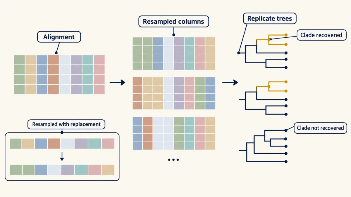
Then comes support. Joseph Felsenstein, in 1985, applied the bootstrap to trees; resampling with replacement means a column can be drawn twice and another left out.
Predict. Suppose the vertebrate tree carries bootstrap values of 98 on (frog, human) and 72 on (trout, (frog, human)). Is the frog-human clade 98% likely to be true?
Check your prediction
No. Those clades appeared in 98% and 72% of the replicate trees. A bootstrap value tells you how consistently the characters in hand recover a clade under the method used. If the model is wrong in a systematic way, the same wrong clade can come back from every replicate.
A simulation with a known true tree showed a poorly fitting model doing exactly that (see Going deeper).
A node with more than two descendant branches, a polytomy, usually means the data were not strong enough to resolve the order of splits. It is rarely evidence that three lineages split at once.
Design problem
Similar twig-dwelling lizards, with short limbs and slender bodies, occur on four Caribbean islands. Design a test that distinguishes one origin of the twig form followed by dispersal between islands from repeated independent origins on each island.
Saved in this browser only.
One way to do it
Sample every lizard species you can on all four islands, plus mainland outgroups, and sequence several genes, not genes or traits used to define the twig ecomorph, or the test becomes circular. Infer the tree by maximum likelihood or Bayesian methods, with bootstrap or posterior support.
One origin plus dispersal, with no later shifts from the twig form to other forms, predicts that the twig species form a single clade. Repeated origins predict that each island’s twig species is nested among species from its own island, with different islands’ twig species in different clades. Map the twig form with the outgroup’s state as ancestral and count the changes each hypothesis needs.
Decide in advance what support you require: a twig clade at bootstrap 50 settles nothing, and strong support that is consistent across genes and methods comes closer. Even then, convergence on a tree is an inference with uncertainty. This is the logic of Losos and colleagues (1998) for Greater Antillean Anolis.
Going deeper
When strong support is wrong
Kapli and Telford (2020) simulated protein data on a known animal tree with sponges branching first, letting the amino-acid mix differ among sites. A model assuming one mix at every site returned the wrong tree in 98 of 100 data sets, usually with high support. The error ran one way: data simulated with comb jellies branching first were recovered correctly every time, even by that simpler model, so the authors argued that strong support for comb jellies first in real data may be this kind of artefact.
The root of the animal tree
Schultz and colleagues (2023) mapped the linkage of genes on chromosomes, using unicellular relatives of animals as outgroups, and reported shared derived linkages grouping sponges with cnidarians, placozoans and bilaterians, which places comb jellies as the sister group of all other animals. Copley (2025) argued that their statistical test overstated the significance of some of those linkages. Read this as a live dispute.
Methods in more detail
Formally, Bayesian inference estimates a posterior distribution of trees and model parameters given the data, the model and a prior. An outgroup is the usual way to root a tree, not the only one: midpoint and clock rooting also exist. Gene-family histories, in which a gene’s tree differs from the species tree, are covered in how signaling evolved.
Your notes
Select any text in the lesson to highlight it or add a note to it. Your highlights and notes are saved in this browser and collected in your notebook.
This browser is not letting the site save anything (a private window or strict privacy settings), so highlights and notes will be lost when you leave the page.
How we measure it
Multiple sequence alignment
Sequences of the same gene from each species are lined up so that each column holds positions thought to descend from one ancestral position. The alignment is itself an inference of homology, and errors in it pass into every tree built from it.
Outgroup comparison and parsimony mapping
A taxon known to lie outside the group of interest is used to root the tree and to judge which state of a character is ancestral. Character changes are then placed on branches so that the total number of changes is as small as possible.
Maximum-likelihood and Bayesian tree inference
A model of how sequences change is used to calculate the probability of the alignment on each candidate tree. Likelihood methods search for the tree that makes the data most probable; Bayesian methods estimate a distribution of trees given the data, the model and a prior.
Nonparametric bootstrap
Alignment columns are resampled with replacement to make many replicate data sets, a tree is inferred from each, and each clade is labelled with the percentage of replicate trees that contain it. The number measures how consistently the data recover a clade, not the probability that the clade is true.
Practice questions on this lesson (3) → MCAT-style, original, each with an explanation
Where this lesson fits
Before thisReview first
- How to Test an Evolutionary ExplanationThis course · Lesson 1
A tree is a hypothesis that can be tested and overturned, which is how this lesson treats it.
After thisStudy next
- Molecular EvolutionThis course · Lesson 5
It turns branch lengths into dates with a molecular clock, which this lesson only mentions.
- Speciation: How Barriers to Gene Flow EvolveThis course · Lesson 7
It explains how lineages split, producing the nodes and sister groups you learned to read here.
- History of Life: Transitions, Extinctions and RadiationsThis course · Lesson 8
It uses trees to place radiations and extinctions in time across the history of life.
Elsewhere on the siteFilms, simulations and method films in other courses
- Build a cladogramSimulation · Biology
You can build a cladogram yourself from shared derived traits and see how branch points are chosen.
- Which Similarities Reveal Relatives?Film · Biology
It shows how shared derived traits locate closest relatives, as a whale's kinship to land mammals does.
Suggested by an AI model from the lessons themselves, then checked. How we use AI
Finish line
Test yourself
8 questions
Practice and MCAT-style, with explained answers.
Next · Lesson 3
Natural Selection in Ecological Context
On lichen-covered trees, birds find dark moths more easily than pale ones. Is that evolution yet, and what else would you need to know?
Continue →