Genetics and Molecular Biology · Unit 6: Populations and complex traits
Population Genetics: Hardy-Weinberg and Evolutionary Forces
Rewritten on : new text, flashcards and film. Your notes and highlights stay, but the text around them may have moved.
If a trait is dominant, why does it not take over a population?
Pause when the reading reaches a film, and offer to play it. Saved on this device.
Watch the film now, or keep listening
Builds on:Probability, Crosses and the Chi-Square TestMendel's Peas: Segregation and Independent AssortmentMutation: Where Variation Comes FromWhy these?
 ▶ Watch Why Dominance Does Not Spread an Allele · 3:34
Read the transcript of “Why Dominance Does Not Spread an Allele”
Film transcript: Why Dominance Does Not Spread an Allele
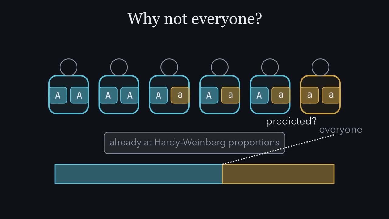
A dominant allele shows its trait whenever a person carries it. Why does it not spread until nearly everyone carries it? Follow the allele copies, not just the visible trait. Their count will expose the answer. Each person holds a genotype, an allele pair at one locus. Population genetics asks a different question. Across everyone, what fraction of all copies are blue? That fraction is an allele frequency. An individual cannot supply that population-wide fraction. The pool contains blue copies and gold copies. Their fractions are called p and q. Together they fill the pool. Dominance changes which pairs show a trait, but it adds no blue copies.
The pool measures inheritance, not outward appearance. Now let eggs and sperm pair at random. Before they pair, predict the next blue fraction. Does random pairing increase it, decrease it, or leave it unchanged? Keep your eye on the copies.
Random means each draw follows the pool's current mix. Draw blue from both lanes, and the pair is a blue homozygote. Draw unlike colours, in either order, and the pair is heterozygous. Draw gold from both, and the pair is a gold homozygote. No draw remembers which phenotype carried a copy. The square gives the expected Hardy-Weinberg genotype proportions.
Blue homozygotes occupy p squared. Heterozygotes occupy both mixed regions. Gold homozygotes occupy q squared. Together the regions fill the whole next generation. These areas describe people, not new allele copies. Recount blue copies in the new people. Every blue homozygote contributes only blue. Every mixed pair contributes half blue. Together those shares return exactly to p. Random mating changed the pairings, not the allele frequency. Dominance still changes the visible count. Both blue homozygotes and heterozygotes show the dominant trait. Yet visibility is not transmission advantage. A visible effect is not a copying mechanism. Without unequal survival, reproduction, or another force, blue copies receive no extra route forward.
This is a baseline, not a claim that real populations are motionless. It assumes a large population, random mating at this locus, and no force changing the copy pool. Hardy-Weinberg predicts genotype counts. It turns no-force reasoning into a testable expectation.
Data can then depart from that expectation. So answer the opening question by counting copies. Mating reshuffles alleles; dominance alone does not change their frequency. A changing allele bar requires something that changes which copies enter the next generation.
From the film
- Mating reshuffles alleles; dominance alone does not change their frequency.
- At a two-allele autosomal locus, allele frequency counts copies across the population.
- With equal allele frequencies in eggs and sperm, random mating gives expected genotype proportions p squared, two p q and q squared.
- Hardy-Weinberg is a null model, not proof that no evolutionary force acts.
Here you calculate the first film’s answer and test it against real counts.
The idea: with nothing acting, frequencies stay put
A population, here, is a group of individuals that mate with one another. At a locus (a place on a chromosome) with two alleles (versions), A and a, the fraction of all allele copies that are A is p and the fraction that are a is q: the allele frequencies. A genotype frequency is the fraction of individuals who are AA, Aa or aa. With two alleles, p + q = 1. (In this lesson p and q are always allele frequencies. The capital P in “P = 0.05” further down is a probability from the chi-square test.)
The one idea. Mating reshuffles alleles; dominance alone does not change their frequency.
Scope: one two-allele autosomal locus in a large population, with the same allele frequencies in eggs and sperm. (In a small population, chance sampling of gametes moves frequencies: that is drift.) The Hardy-Weinberg baseline below adds random mating at this locus and no selection, mutation or migration.
Written as algebra, the first film’s square gives the Hardy-Weinberg proportions:
In words The AA share is p squared, the Aa share is two times p times q, the aa share is q squared, and the three shares add up to everyone.
- p2“p squared”
- the expected frequency of AA: draw A from the egg and A from the sperm, p × p
- 2pq“two p q”
- the expected frequency of Aa: A from the egg and a from the sperm (pq), or the reverse (qp)
- q2“q squared”
- the expected frequency of aa, q × q
- p“p”
- the frequency of allele A: the fraction of all allele copies in the population that are A
- q“q”
- the frequency of allele a. With two alleles, q = 1 − p.
Sanity check If q = 0 there are no a copies, and the equation says everyone is AA (p2 = 1). If p = q = 0.5, heterozygotes make up half the population (2 × 0.5 × 0.5 = 0.5), the most they ever can at two alleles.
Try one number
Take q = 0.10, so p = 0.90.
AA: 0.90 × 0.90 = 0.81. Aa: 2 × 0.90 × 0.10 = 0.18. aa: 0.10 × 0.10 = 0.01.
Check the total: 0.81 + 0.18 + 0.01 = 1.00. With an allele at 10%, only 1 person in 100 is aa, but 18 in 100 carry one copy.
Need a refresher? powers and roots
This is the product and sum rule from probability and crosses, applied to a whole population. The first film’s recount of A copies, in three lines (AA zygotes are all A; Aa zygotes are half A):
- A frequency = p2 + (half of 2pq) = p2 + pq.
- Take p out of both terms: p2 + pq = p(p + q).
- p + q = 1, so this is just p.
The allele frequency has not moved, and one generation of random mating gives these genotype proportions whatever the proportions were before, provided eggs and sperm begin with the same p and q.
G. H. Hardy published this in 1908; Wilhelm Weinberg, a physician in Stuttgart, derived it independently in a lecture in January 1908, so the principle carries both names. W. E. Castle and Karl Pearson had made earlier attempts at the same problem.
Hardy-Weinberg is a null model: what you would see under the baseline in the box above, against which you detect departures. Real populations break its assumptions.
Counting alleles and testing equilibrium
Worked problem, part 1. In a sample of 1,000 people typed at a codominant locus (each genotype distinguishable), there are MM 298, MN 489 and NN 213. Assume unrelated individuals and accurate typing.
- Count alleles, not people. Each MM person carries two M copies and each MN person one. M copies = 2 x 298 + 489 = 1,085, out of 2,000. So p = 0.5425, and q = 1 - p = 0.4575. Count first; never find p from the square root of a homozygote frequency before you know the sample is at equilibrium.
- Expected counts. Multiply the sample size by each Hardy-Weinberg proportion. MM = 1,000 x 0.54252 = 294.3. MN = 1,000 x 2 x 0.5425 x 0.4575 = 496.4. NN = 1,000 x 0.45752 = 209.3. They add to 1,000.
- Chi-square, a score for how far the counts sit from the expected ones (bigger means more surprising; see probability and crosses). (298 - 294.3)2 / 294.3 = 0.046; (489 - 496.4)2 / 496.4 = 0.110; (213 - 209.3)2 / 209.3 = 0.065. The total is 0.22.
- Degrees of freedom. Three classes, minus 1 because the counts must add to 1,000, minus 1 more because p was estimated from these same counts: 1, not 2.
- Decide. The critical value at P = 0.05 for one degree of freedom is 3.84. Since 0.22 is far below it (P is about 0.64), there is no evidence of departure.
That is all: a good fit does not prove random mating or the absence of selection, and a poor fit does not prove selection, because inbreeding, a sample that mixes two populations, and genotyping errors can all produce one.
Worked problem, part 2. A recessive condition affects 1 in 2,500 newborns in a hypothetical population. Assume the population is at equilibrium at this locus.
Predict. Will carriers be nearer 1 in 2,500, 1 in 50 or 1 in 25? Name their Hardy-Weinberg term.
Check your prediction
Carriers are two p q, about 1 in 26, so 1 in 25 is the closest choice.
Affected people are aa, so q2 = 1/2,500; the square root gives q = 1/50 = 0.02, and p = 0.98. Carriers are 2pq = 2 x 0.98 x 0.02 = 0.039, about 1 in 26 (1 ÷ 0.0392 is about 25.5).
Carriers are about 100 times as common as affected people (0.0392 / 0.0004 = 98). In symbols, 2pq / q2 = 2p/q (one q cancels), and when q is small p is close to 1, so the ratio is close to 2/q: here 2/0.02 = 100. A rare allele sits almost entirely in heterozygotes: here 98% of a copies are in carriers. This is how families meet a recessive condition with no affected relatives in the pedigree.
That 1 in 26 needs both q = 0.02 and Hardy-Weinberg proportions: non-random mating can change it while q stays fixed. The second film asks what can move q.
Read the transcript of “What Moves Allele Frequencies?”
Film transcript: What Moves Allele Frequencies?
The first film left the blue and gold allele bar unchanged after mating. What must happen to move that boundary? Keep following copies as different processes act on the population. The answer depends on what touches those copies.
Selection acts when genotypes leave different numbers of surviving offspring. Suppose a genotype contributes fewer copies to the next pool. The bar moves predictably toward the copies contributed more often. Which genotype has that advantage depends on the environment. So the direction can change when the environment changes. Migration moves copies between populations. Pour a small stream from a population with a different allele mix into the resident pool. The new frequency becomes a weighted average. It shifts toward the migrants' mix. The amount of movement depends on the migrants' share. Mutation changes the identity of a copy. A blue block flips to gold as it enters the next pool.
That creates a new route between allele states. At a human locus, the immediate frequency change is usually weak. Mutation supplies variation on which other forces act. Now copy the same small population twice. Each copy samples its next generation by chance. Both begin with the same copy inventory.
Predict the result. Must both allele bars move together, or can identical starting populations separate without selection? They can separate. Drift is random sampling of allele copies between generations. One sample happens to take more blue; another takes more gold.
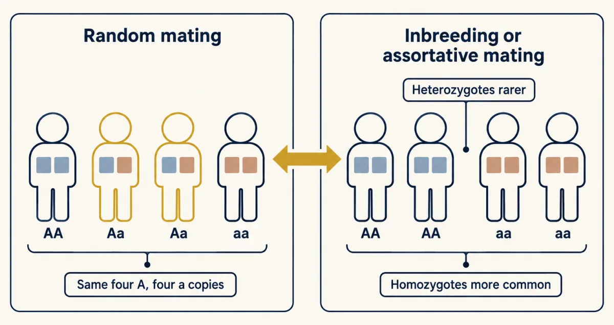
Across many repeats there is no preferred direction, but small populations spread widely. Non-random mating produces a different signature. Relatives, or partners alike in a trait this locus affects, pair more often. So homozygotes can increase while heterozygotes decrease. Yet every blue and gold copy remains. The bar therefore stays in the same place. Mating pattern alone changes genotype frequencies, not allele frequencies. These processes can overlap, so an unusual sample rarely names a cause. A heterozygote deficit might reflect non-random mating, mixed populations, or genotyping error. A pattern can therefore support several explanations.
Population genetics compares predictions with patterns, then asks for independent evidence. Track what each process touches. Selection changes contribution. Migration changes membership. Mutation changes identity. Drift changes the sample. Non-random mating changes pairing. The moving bar is evidence to explain, not a label for one cause. Forces change allele frequencies in distinct, testable ways. Follow the copies, compare the expected signature with the data, and keep alternative causes open until more evidence separates them.
From the film
- Forces change allele frequencies in distinct, testable ways.
- Selection changes which genotypes contribute copies; migration mixes populations.
- Mutation creates alleles, while drift samples them without a preferred direction.
- Non-random mating alone rearranges genotypes without changing allele frequencies.
What can move a frequency?
The second film showed what each process touches; here is how far and how fast. Recall the rule: mating reshuffles alleles; dominance alone does not change their frequency. To move a frequency, something has to act on the population.
Selection (genotypes differing consistently in survival or reproduction) is fast or slow depending on which genotypes it can “see.” Against a rare recessive it is slow, because selection acts only on aa, and almost every a copy is hidden in a carrier. If aa individuals never reproduced, q would fall as qn = q0 / (1 + n q0), where q0 is the starting frequency and qn the frequency after n generations. Starting at 0.02, halving q to 0.01 takes 50 generations: with qn = 0.01, 1 + n × 0.02 must equal 0.02 / 0.01 = 2, so n = 50. (Check: at n = 0 the formula gives q0, and q shrinks ever more slowly as it gets rarer.)
Migration (gene flow) gives the second film’s weighted average.
Predict. Residents have p = 0.2, migrants p = 0.6, and migrants supply one tenth of the copies. Estimate the new p.
Check your prediction
Nearer 0.2, because residents supply nine tenths of the copies.
In words Next generation's p is the residents' share times their frequency, plus the migrants' share times theirs.
- p'“p prime”
- the frequency of allele A in the next generation
- m“m”
- the fraction of the next generation's allele copies that come from migrants, so 1 − m come from residents
- p“p”
- the residents' frequency of A now
- pm“p sub m”
- the frequency of A among the migrants
Sanity check With no migrants (m = 0) p' = p and nothing changes. If every copy came from migrants (m = 1), p' = pm. Between those, p' always lands between p and pm.
Try one number
With p = 0.2, pm = 0.6 and m = 0.1: residents supply 0.9 × 0.2 = 0.18 and migrants supply 0.1 × 0.6 = 0.06.
p’ = 0.18 + 0.06 = 0.24. The frequency moved a tenth of the way from 0.2 toward 0.6, because a tenth of the copies are new.
Need a refresher? subscripts and Greek letters
Mutation, the source of new alleles (see mutation), is weak on frequency. In human parent-offspring trios, the TOPMed study estimated about 1.2 x 10⁻⁸ new single-base changes per base pair per generation, a genome average. That is about one change per 83 million base pairs (1 ÷ 1.2 x 10⁻⁸ is about 83 million; see powers). Over a few generations, that barely moves an allele frequency.
Non-random mating is the odd one out, as the second film showed: same copies, different pairs. Its two kinds are inbreeding (mating between relatives) and assortative mating (partners alike in a trait the locus affects). By putting more rare recessive copies into aa individuals, they can still expose those alleles to selection.
Drift and founders: chance in small populations
The second film’s two cups showed drift: chance sampling of the parents’ allele copies. Under the simplest model, with a constant effective population size Ne (the number of breeders in an idealized population that would drift at the same rate), one generation’s wobble has a known size.
Predict. At the same Ne, is one-generation variance larger at p = 0.5 or p = 0.1? Check the boundaries.
Check your prediction
Larger at p = 0.5; p(1 - p) peaks halfway between the boundaries.
In words The variance of the change in p equals p times one minus p, divided by twice the effective population size.
- Δp“delta p”
- the change in the allele frequency p from one generation to the next. Var(Δp) is its variance: how widely that change scatters if you could rerun the generation many times.
- p“p”
- the allele frequency now
- Ne“N sub e”
- the effective population size. Each breeder passes on two allele copies, hence the 2.
Sanity check If p is 0 or 1 the variance is zero: a lost or fixed allele has nothing left to drift. The wobble is largest at p = 0.5, and it shrinks as Ne grows, so drift matters most in small populations.
Try one number
With Ne = 50 and p = 0.5: the top is 0.5 × 0.5 = 0.25 and the bottom is 2 × 50 = 100.
Variance = 0.25 / 100 = 0.0025. The standard deviation is its square root, 0.05.
Across repeated populations, the one-generation changes have standard deviation 0.05. Any one population can move less or more, in either direction.
Need a refresher? powers and roots
Left long enough, a small population’s frequency wanders until it hits 0 (the allele is lost) or 1 (it is fixed).
| Expected | Observed |
|---|
With no systematic force acting, the expected p stays put; drift scatters small populations around that line without a direction, and selection gives the line one. This is a sketch of the logic: constant Ne, random mating, selection against aa only. Viability selection with wAA = wAa = 1 and waa = 1 - s; each generation draws 2Ne allele copies at random (binomial sampling); 30 replicates, 50 generations. Here s is the cost to aa, not the s of q = s/(s + t).
Peter Buri saw this in 1956 in 107 laboratory populations of Drosophila, each kept at 8 males and 8 females and started at one half for an eye-colour allele. Over 19 generations they spread apart and many lost or fixed the allele, while their average stayed near where it began.
A founder effect is drift at the start of a population: a small group carries, by chance, a different set of alleles than the population it left. In a 2020 exome study of 5,521 Lancaster County Old Order Amish participants, 124 carried the KCNQ1 variant p.T224M, about 1 in 45, and none was homozygous. Each person carries two copies, so the 124 carriers hold 124 variant copies out of 2 x 5,521 = 11,042, an allele frequency of about 0.011: a carrier frequency of 1 in 45 is not an allele frequency of 1/45. The authors note that pathogenic variants may occur at much higher frequency in founder populations, and they attribute this variant’s frequency to a founder effect and drift. Tay-Sachs disease among Ashkenazi Jewish people and the rare diseases of the Finnish disease heritage are other examples often taught this way. These are features of particular populations and their histories, not of races: most human genetic variation lies within populations, not between them.
Balanced polymorphism: sickle cell and malaria
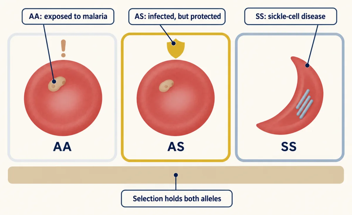
The sickle allele of the β-globin gene (HBB) changes glutamate to valine at position 6 of the β chain, and deoxygenated HbS polymerises (see protein binding and allostery). Sickle-cell disease (SS) is autosomal recessive. In conditions where the disease shortens life, selection should remove S. Yet in regions with intense falciparum malaria the allele is common.
Predict. If AS survives better than both homozygotes, should S disappear, become fixed, or settle between?
Check your prediction
Between the extremes: rare S sits mostly in favoured AS, while common S makes more SS, which selection removes.
The reason is heterozygote advantage. In two cohorts of children on the Kenyan coast, sickle-cell trait (AS) made no difference to how often children carried parasites without symptoms, but it was associated with about 50% protection against mild malaria, 75% against hospital admission and almost 90% against severe disease. The allele settles where the losses at the two homozygotes balance; with costs s to AA and t to SS, the equilibrium is:
In words The equilibrium frequency of S is the cost to AA divided by the two costs added together.
- q“q”
- the frequency of the S allele at equilibrium
- s“s”
- the fitness cost to AA homozygotes: 1 minus their survival relative to AS
- t“t”
- the fitness cost to SS homozygotes: 1 minus their survival relative to AS
Sanity check If the two costs are equal (s = t), q = 1/2. If SS costs far more than AA (t much bigger than s), q is small: the allele stays rare because each S copy that lands in an SS person is lost. If AA paid no cost (s = 0), q = 0 and nothing would hold S.
Try one number
Round values to keep the arithmetic easy (not data): s = 0.2 and t = 0.8.
q = 0.2 / (0.2 + 0.8) = 0.2 / 1.0 = 0.2.
So S would settle at 20% of allele copies, with A at 80%.
Need a refresher? rates and “per”
Design problem
Interpret these illustrative data (not measurements) for a malaria-endemic population. Newborns are AA 0.81, AS 0.18 and SS 0.01, so q = 0.10, at Hardy-Weinberg proportions. Relative survival to adulthood is AA 0.88, AS 1.00 and SS 0.20. What maintains the S allele, where should its frequency settle, and what would adults look like? What other data would you need to rule out migration or drift?
Saved in this browser only.
One way to do it
Heterozygotes survive best, so this is balancing selection. The fitness costs are s = 1 - 0.88 = 0.12 for AA and t = 1 - 0.20 = 0.80 for SS. Assuming a large, randomly mating population with survival as the only force, the equilibrium is q = s / (s + t) = 0.12 / (0.12 + 0.80) = 0.12 / 0.92 = 0.13. Since newborns start at 0.10, q should rise slightly over generations.
Check one generation. Survivors are AA 0.81 x 0.88 = 0.713, AS 0.18, SS 0.01 x 0.20 = 0.002, out of 0.895. As fractions of adults: AA 0.797, AS 0.201, SS 0.002. Adult q = 0.201/2 + 0.002 = 0.103. Under Hardy-Weinberg, q = 0.103 predicts 2 x 0.897 x 0.103 = 0.185 heterozygotes, but adults have 0.201. Adults show a heterozygote excess, even though their newborns fit. When to sample matters.
To separate selection from the alternatives, show that the allele’s frequency follows the historical intensity of malaria across regions, that AS children are protected in follow-up studies, and that newborns fit equilibrium while adults show the excess. Migrants from a high-S population would raise q, but if they come from a population at Hardy-Weinberg proportions the mixture shows a heterozygote deficit, not an excess, unless the adult migrants were themselves selected in a malarious region; so record where each adult was born.
The next lesson uses the same allele counts, across hundreds of thousands of loci at once, to look for variants associated with complex traits.
Your notes
Select any text in the lesson to highlight it or add a note to it. Your highlights and notes are saved in this browser and collected in your notebook.
This browser is not letting the site save anything (a private window or strict privacy settings), so highlights and notes will be lost when you leave the page.
How we measure it
Gene counting and the Hardy-Weinberg chi-square test
Each genotype is counted, and allele frequencies are found by counting allele copies, with no assumption about equilibrium. Expected counts under Hardy-Weinberg proportions are then compared with the observed ones, by a chi-square with one degree of freedom or by an exact test when an allele is rare.
Hemoglobin electrophoresis
Hemoglobin from a blood sample is run through a gel in an electric field. HbS has lost one negative charge on each beta chain, so it moves differently from HbA, and carriers (AS) show both bands. This lets a survey count AA, AS and SS individuals directly.
Replicate small populations
Many populations are started from the same allele frequency and kept at a fixed small size. Chance acts differently in each, so the spread of frequencies across populations shows drift directly, which a single population cannot.
Exome sequencing in a founder population
The protein-coding parts of the genome are sequenced in thousands of members of a population descended from few founders. Variants that drift made common can be counted and tested for association with a trait, and then tested for function in cells.
Practice questions on this lesson (3) → MCAT-style, original, each with an explanation
Where this lesson fits
Before thisReview first
- Probability, Crosses and the Chi-Square TestThis course · Lesson 3
You need the product and sum rules and the chi-square test from there to derive and test Hardy-Weinberg proportions.
- Mendel's Peas: Segregation and Independent AssortmentThis course · Lesson 1
Segregation of two alleles into equal gametes is what lets random mating give p squared, 2pq and q squared.
- Mutation: Where Variation Comes FromThis course · Lesson 14
Mutation as the source of new alleles is the force you weigh against selection and drift here.
After thisStudy next
- Complex Traits, Heritability and GWASThis course · Lesson 26
It uses the same allele counts and frequencies across many loci to link variants to complex traits.
Elsewhere on the siteFilms, simulations and method films in other courses
- The Drought Sorts a PopulationFilm · Biology
It shows selection sorting inherited traits in a real population, the force that changes allele frequencies here.
- How Populations ChangeFilm · Biology
It shows how mutation, gene flow and selection change allele frequencies across generations, as in the forces discussed here.
- Mean and SpreadFilm · Ecology and Evolution
It shows drift as chance sampling of parents' alleles, with migration moving the mean and drift spreading replicate populations.
- Selection Has an AgentFilm · Ecology and Evolution
It shows selection as unequal reproductive success caused by an environmental agent, as with malaria and the sickle allele.
Suggested by an AI model from the lessons themselves, then checked. How we use AI
Finish line
Test yourself
8 questions
Practice and MCAT-style, with explained answers.
Next · Lesson 26
Complex Traits, Heritability and GWAS
If height is 80 percent heritable, does that mean 80 percent of your height came from your genes?
Continue →← Lesson 24 · Forward and Reverse Genetics: Screens, RNAi and CRISPR