Ecology and Evolution · Unit 1: Evidence and evolutionary reasoning
New to this? Review it at high school level: Variation and Survival, Natural Selection and New Species
Drift, Gene Flow and Competing Explanations
Rewritten on : new text, flashcards and film. Your notes and highlights stay, but the text around them may have moved.
Sixteen flies bred each generation, yet the flies drifted as if there were only nine. Why?
Pause when the reading reaches a film, and offer to play it. Saved on this device.
Watch the film now, or keep listening
Builds on:How to Test an Evolutionary ExplanationNatural Selection in Ecological ContextWhy these?
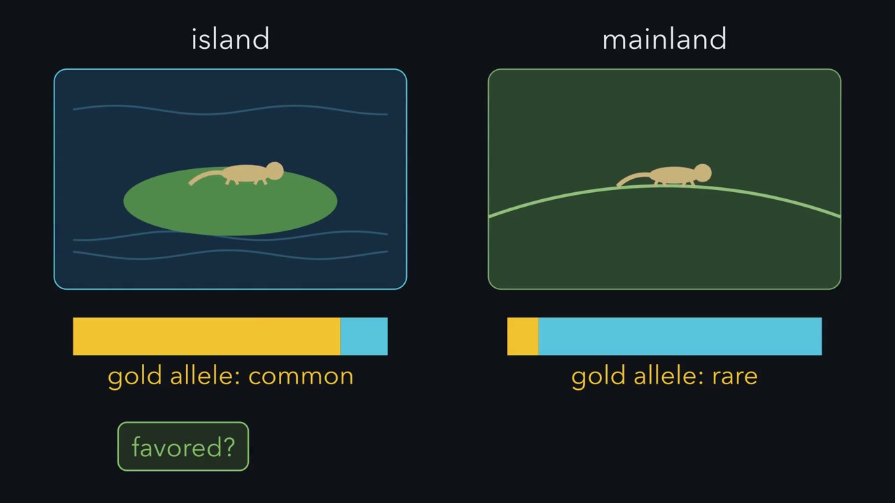 ▶ Watch Mean and Spread · 3:27
Read the transcript of “Mean and Spread”
Film transcript: Mean and Spread
An allele is common on an island and rare on the mainland. Did something favour it there, or was it luck? Or did migrants bring it? Picture one generation's gene pool as a bag of beads. Gold beads carry one allele, and blue beads carry the other. Half of them are gold. To make the next generation, a hand draws beads at random, and puts each one back after noting its colour. A small draw is rarely a perfect copy of the bag. This one came out heavy on gold. Nobody chose gold. The sample was just small. Change in allele frequency from chance sampling of parents is called genetic drift. It needs no difference in fitness. One bag tells you little.
So run many bags side by side, all starting half gold. Each bag is a replicate population. Generation after generation, each bag wanders on its own. Some climb and some fall. A few reach all gold or all blue, and then they stay there. Now watch the white triangle. It marks the average across all the bags. The bags spread apart, but the triangle stays close to where it started. That is drift's signature across replicates. It spreads them apart without pushing their average. Chance favours no direction, so the triangle only wobbles. Now make every bag ten times bigger, and start again. The dots still spread, but far more slowly. Bigger pools scatter less.
What sets the scatter is not simply the number of animals you count. It is the effective population size, the size of an ideal population that drifts as fast. Back to small bags, all half gold. Now pour beads from outside into every bag, mostly blue ones. That is gene flow. Every bag started at one half and got the same pour. So every dot slides the same distance toward the immigrants. The triangle slides with them. Unlike drift, this happens the same way every time. Last, let gold carriers leave slightly more offspring, in every bag. That is consistent selection. What happens to the triangle? And what happens to the spread?
The triangle creeps toward gold, so consistent selection pushes the average. But while both alleles remain, the dots keep scattering around it. Here is the test. Compare the replicate average with what chance alone would give. Then, for selection, check whether carriers really do better. For gene flow, track the migrants. One population's frequency, on its own, cannot tell luck from cause.
Replicates give it an average to compare with.
From the film
- Genetic drift is change in allele frequency from the chance sampling of parents; it needs no difference in fitness.
- Across replicate populations, drift spreads allele frequencies apart without pushing their average.
- Gene flow pulls replicates that start alike and receive the same immigrants toward the immigrants' frequency by the same amount.
- Consistent selection, favouring the same allele everywhere, pushes the average toward it, while drift still scatters each population.
- How fast the replicates spread depends on the effective population size, Ne, not simply the number of animals you count.
The first film built the rule with bags of beads; this text adds its limits, the size of the scatter, and real populations. The key tool is replicate populations: populations started at the same allele frequency and kept alike, so chance shows up as a spread among them.
The one idea. Across replicate populations, drift spreads allele frequencies apart without pushing their average; gene flow and consistent selection push the average. So to tell the forces apart, compare the replicates’ average with a neutral null (what chance alone predicts), then test selection with an independent fitness assay and gene flow with measures of immigration and ancestry.
Scope: one locus (a position or region in the genome), two alleles, replicates that start alike in one setting. “Without pushing” means the expected average stays put; a finite set of replicates still wobbles, with no trend. Gene flow moves each population a fraction m of its distance from the immigrants’ frequency pm, so with the same m and pm, populations that start alike move alike and populations that have drifted apart do not. Consistent selection favours the same allele in every replicate. One population’s frequency, on its own, cannot tell luck from cause, and an unchanged average does not exclude selection (Going deeper). This scope holds wherever the rule appears below.
Drift is sampling error
The first film’s bead draw stands for two chance steps in a real population: which of a parent’s two copies goes into each egg or sperm, and how many offspring each parent leaves. The resulting change in allele frequency is genetic drift. It needs no difference in fitness (the relative number of surviving offspring an individual leaves in a given environment), so it acts on all alleles alike and can carry a harmful allele up or a beneficial one to loss, especially in small populations.
The textbook model of a closed, ideal population is the Wright-Fisher model (assumptions in Going deeper): N diploid individuals carry 2N gene copies, and each generation’s 2N copies are drawn at random from the parents’ pool. A bigger sample is a closer copy of the pool, so the scatter shrinks as 2N grows:
In words On average the frequency stays where it was; the variance is p times one minus p, divided by the number of gene copies sampled.
- p“p”
- the allele's frequency among the parents
- 1 − p“one minus p”
- the other allele's frequency
- 2N“two N”
- gene copies sampled: two per diploid individualcopies
Sanity check As 2N grows without limit the scatter goes to zero. At p = 0 or 1 it is also zero: a fixed allele cannot drift.
Need a refresher? reading an equation · powers and roots
Predict. A neutral allele sits at 0.60. If drift runs until only one allele is left, how often will this one be the survivor?
Check your prediction
60% of the time. Far enough in the future, every copy of the gene descends from a single copy alive now. Under neutrality that ancestor is a random pick, and 60% of today’s copies carry this allele. So a neutral allele’s chance of fixing, reaching frequency 1, equals its current frequency; at 0.60 it is lost 40% of the time. Population genetics in the Genetics course works through the algebra.
Real populations drift faster than their census size N, the head count, suggests: if a few parents leave most of the offspring, the next generation samples only those few, and an uneven breeding sex ratio or a size that swings from year to year does the same. So drift is scaled by the effective population size (Ne), the size of the ideal population that drifts as fast, usually below N.
A bottleneck is a sharp drop in numbers that leaves a chance sample of the original gene pool. A founder effect occurs when a new population starts from a few individuals who carry an unrepresentative sample of their source population’s variation.
Worked problem (illustrative numbers). A neutral allele has frequency 0.60 in a resident population and 0.20 among immigrants. After migration, immigrants make up m = 0.10 of the breeding pool. The next generation is 100 diploid offspring, so 2N = 200 gene copies are sampled, with no selection, no mutation and no further migration during sampling.
- Migration. The mixed frequency is a weighted average: p = 0.90 x 0.60 + 0.10 x 0.20 = 0.54 + 0.02 = 0.56. Gene flow shifted the frequency by 0.56 - 0.60 = -0.04, a deterministic shift, the same every time.
- Drift’s expected outcome. 200 x 0.56 = 112 copies, a frequency of 0.56; drift adds no push.
- Scatter from drift. The variance is 0.56 x 0.44 / 200 = 0.2464 / 200 = 0.001232. Variance is in squared units, so take its square root, the standard deviation, to get the scatter in frequency units: 0.035, about 3.5 percentage points.
Predict. Cut the offspring tenfold, to 10 (2N = 20 copies). Is the scatter ten times bigger?
Check your prediction
No, about three times (the square root of 10 is 3.16). The variance, 0.2464 / 20 = 0.01232, is ten times bigger, but the standard deviation is its square root: 0.111, about 11 points.
| Expected | Observed | |
|---|---|---|
| Mean offspring frequency | ||
| Standard deviation | ||
| Copies of the allele out of 2N |
In this sketch: one generation; neutral Wright-Fisher, with 2N gene copies drawn at random from the mixed pool; no selection, no mutation, no further migration during sampling; resident 0.60 and immigrant 0.20 are the lesson’s illustrative numbers. m (0 to 0.5) and N (10 to 200) are free settings here; the lesson works m = 0.10 with N = 100 and N = 10. 500 resamples is this sketch’s choice; the lesson says “many times”.
Migration moves the mean, deterministically; drift spreads the outcomes around it, in neither direction, and the spread shrinks as the number of gene copies grows. This is a sketch of the logic, not a prediction for a real population.
One generation in one population gives a single draw from that scatter. To see the scatter itself you need many populations at once, which is what Buri built.
Read the transcript of “107 Bottles”
Film transcript: 107 Bottles
To see drift's scatter, you need many populations at once. Do real animals spread apart like the beads, with their average left alone? From one bottle's frequency alone, you could not tell. Follow one line alone. It climbs, dips and climbs again. Was it pushed, or was it luck? Peter Buri published the real experiment, with fruit flies. He followed two alleles of a gene for eye colour, the brown locus. Every line started at one half gold. Each generation, he picked sixteen flies as the parents of the next. His first series had a hundred and seven lines. Every bottle was set up the same way and kept the same way. So chance alone predicts differences between the lines.
Now stack all the lines into one picture. Each bar counts how many lines sit at each frequency. At the start, every line is in the middle bar. Generation by generation, the pile flattens. Lines drift up and down. Some lose blue entirely, some lose gold, and those stay at the edges. By generation ten, the edges are filling up. Now watch the white triangle, the pooled frequency across all lines. By generation nineteen, will it be up, down, or still at one half?
Still at about one half. By then many lines had ended with only one allele. Yet the pooled frequency showed no systematic change. Spread without a push on the average. That is the pattern drift predicts, now seen in real flies rather than beads. But how fast did the lines spread?
Buri asked how big an ideal population would have to be to spread that fast. Here is the spread computed for an ideal population of sixteen. Buri's real lines spread faster than that, with more of them at the edges. From how fast his own lines spread, Buri estimated about nine. They drifted as if each bottle held only nine flies. That number is the effective population size, Faster spread means a smaller effective size. It measures how hard chance acted, not how many flies were in the bottle. So one line wanders, and tells you little about cause. Many replicates, side by side, show whether the average was pushed.
From the film
- Buri started 107 fruit-fly lines at an allele frequency of 0.5 and kept 16 parents in each, generation after generation.
- Over 19 generations the lines spread toward 0 and 1, and many ended with only one allele.
- The frequency pooled over all the lines showed no systematic change: spread without a push on the average, the pattern drift predicts.
- From how fast the lines spread, Buri estimated an effective size of about 9, below the 16 flies in each bottle.
- One line on its own wanders and tells you little about cause; replicates show whether the average was pushed.
Buri’s 107 fly lines: drift as a distribution
Two things the second film left out: how firm its reading is, and why nine.
The pattern is consistent with drift rather than proof of it; Buri also compared the changes with what sampling alone predicts and found no evidence of selection. His Ne of 9.0, estimated from how fast the lines spread apart, is the mean for his first series. Buri said the cause of the gap was not known, but judged that variation in how many offspring each fly left, down to complete sterility, was certainly part of it, and thought crowding for egg-laying space in the small vials probably played a role.
Founders and frontiers: anoles on islands, bacteria on agar
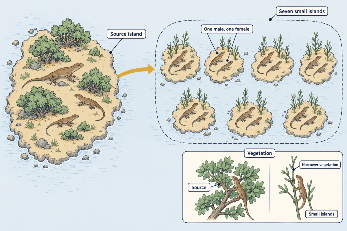
Founder effects in nature are usually reconstructed after the fact; Jason Kolbe, Jonathan Losos and colleagues made them happen, releasing one randomly drawn male-female pair of brown anoles, Anolis sagrei, from a single source island onto each of seven small islands in the Bahamas, where the vegetation was narrower than on the source.
Predict. One source, random founders, narrow perches everywhere: will the island populations come to look alike, stay different, or both?
Check your prediction
Both. The 2012 report in Science found that genetic and morphological differences that tracked the founding pairs persisted throughout the experiment: that is the spread. And all the populations evolved shorter hindlimbs, the direction predicted for lizards on narrow perches: a shared shift in the average, the pattern selection predicts.
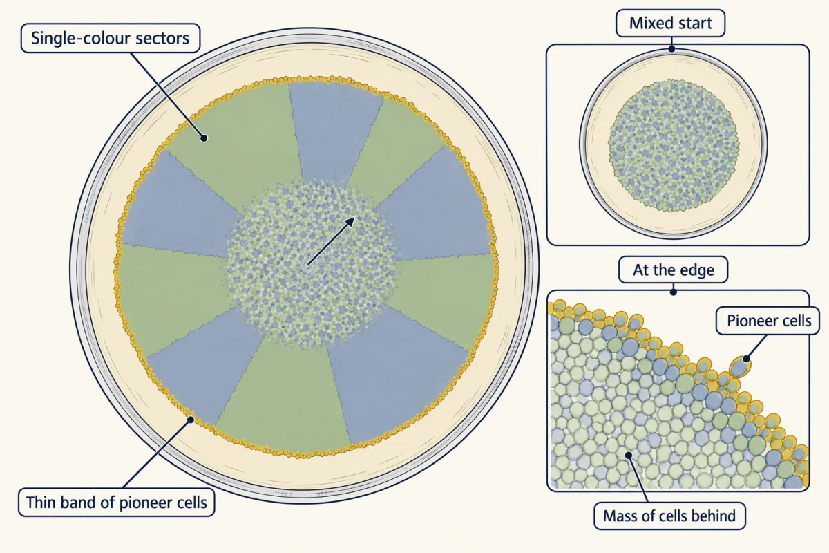
Large populations drift too. Oskar Hallatschek and colleagues (2007, PNAS) mixed two Escherichia coli strains that differed only in a fluorescent label and let the colony spread across agar. It broke into single-colour sectors, because chance in the thin band of pioneer cells at the edge decided which colour got carried outward: a spreading front is a series of founder events. As with Buri’s flies, the head count is not what chance acts on.
Gene flow: swamping or rescue
Gene flow is the movement of alleles between populations by individuals or gametes, pollen included. Beyond the first film’s matched bags, each population moves by m × (pm − p), a fraction m of its distance from the immigrants’ frequency pm (step 1 of the worked problem). With m = 0.10 and pm = 0.20, a population at 0.30 moves to 0.29 and one at 0.70 to 0.65: populations that had drifted apart move by different amounts, and the gap shrinks from 0.40 to 0.36. Two-way exchange also pulls populations together.
It can harm. Migration load is a drop in a population’s mean fitness caused by immigrant alleles that suit somewhere else. Timema cristinae walking-sticks live on two host plants, and colour morphs differ in how well they are camouflaged on each. Daniel Bolnick and Patrik Nosil (2007, Evolution) compared 25 natural populations and found that those receiving more immigrants from the other host were more poorly matched, and that these showed larger within-generation shifts in morph frequency from selection. It is a correlation that fits the migration-load prediction, not a manipulation of migration.
Predict. Two small, isolated guppy populations in Trinidad start receiving immigrants. Will their fitness fall, as the walking-sticks’ did?
Check your prediction
No, it rose. In the Caigual and Taylor streams, gene flow began after fish from a different source were introduced upstream. Sarah Fitzpatrick and colleagues (2020, Current Biology) followed the recipients with pedigrees. Both populations grew nearly tenfold, and on average hybrids lived longer and reproduced more than residents or immigrants, though in some comparisons hybrids and pure immigrants did about equally well.
That makes this genetic rescue: a rise in a small population’s fitness or growth caused by the genetic effects of gene flow, not just by extra bodies (demographic rescue); the fit hybrids in the pedigrees point to a genetic cause. Nor did the immigrants simply replace the residents: alleles putatively associated with local adaptation were not entirely swamped.
Help can also come from another species: introgression is the movement of alleles from one species into another through hybridization followed by backcrossing, hybrids mating back into the receiving species. In the Houston Ship Channel and Galveston Bay region of Texas, Gulf killifish in polluted water carry tolerance-associated variants that Oziolor and colleagues (2019, Science) inferred had entered by introgression from Atlantic killifish: gene flow supplied the variation, and strong selection raised it.
Whether gene flow harms or helps depends on what the incoming alleles do in their new home.
Three explanations for one pattern
Back to the island allele. Drift spreads replicates without pushing their average; gene flow and consistent selection push it. Each leaves its own signature:
| Explanation | Replicate populations in the same setting | Fitness assay |
|---|---|---|
| Drift alone (the neutral null) | Scatter both ways; the average stays near the starting frequency | Carriers do no better (the model assumes equal fitness) |
| Gene flow | Frequencies track the amount and source of immigration | Not the test: measure immigration and ancestry |
| Consistent selection | The average shifts toward the favoured allele; drift still scatters each one | The favoured genotypes do better (for a recessive allele, only its homozygotes) |
The neutral null can be Wright-Fisher or a colony model, and the independent fitness assay must not rely on the pattern itself. Often the answer is drift and selection together, as with the anoles. The lessons on testing an evolutionary explanation and selection in ecological context use the same logic.
Design problem
In expanding bacterial colonies, one fluorescent strain forms large sectors. Is it fitter, or did it get lucky at the frontier? Design the experiment.
Saved in this browser only.
One way to do it
Grow many replicate colonies from one starting mix, say 20 at 50:50. Under the neutral expectation Weinstein and colleagues (2017, PLOS Computational Biology) used, large sectors in a few colonies are what drift produces; a consistent shift in the mean fraction, beyond what a neutral model calibrated to your colonies allows, is evidence of selection.
Then remove two confounds: swap the fluorescent labels and repeat, so any cost of carrying a marker shows up; and measure each strain’s expansion speed growing alone, an independent fitness assay that does not depend on the sectors.
Keep the scope: Weinstein and colleagues found that some strains ranked differently on agar than in well-mixed liquid culture. A strain that wins on a plate has been shown to win on a plate.
Going deeper
The Wright-Fisher assumptions
A closed population of N diploid individuals, constant in size, with non-overlapping generations, random mating, no selection, no mutation and no migration. Real populations break these, which is why Ne differs from N.
Drift erodes variation
In the neutral Wright-Fisher model with no mutation or migration, expected heterozygosity (the chance that two gene copies drawn at random differ; under random mating, the expected share of heterozygous individuals) falls each generation, faster when Ne is small, though one population’s can wobble. Mutation and balancing selection can maintain it. So small, isolated populations lose variation, which gene flow can restore.
When does selection beat drift?
A rough rule: when Ne multiplied by the selection coefficient s (an allele’s proportional fitness advantage or cost) is well below 1, drift dominates; when it is well above 1, selection does. Do not read 1 as a sharp crossover: in the standard additive model, a new beneficial allele with Ne × s = 1 is already about four times as likely to fix as a neutral one. With few replicates, weak selection can hide inside the average’s chance wobble; more replicates, or more generations sampled through time, raise the power to detect it but do not guarantee it.
Selection that leaves the average alone
Balancing selection, such as a heterozygote advantage whose balance point is the starting frequency, can hold the replicate average still while keeping the spread narrower than drift alone would.
When there are no replicates
For a single island or introgression event, a time series, a genome-wide neutral null, migration estimates and fitness assays can still test whether chance alone explains the pattern.
Where Buri’s design came from
Buri, publishing in 1956, ran a large version of a laboratory design that Warwick Kerr and Sewall Wright had introduced in 1954, using Drosophila melanogaster and two alleles at the brown eye-colour locus.
Founders and new species
Whether founder effects alone can produce new species is debated, and the anole experiment did not test that.
Your notes
Select any text in the lesson to highlight it or add a note to it. Your highlights and notes are saved in this browser and collected in your notebook.
This browser is not letting the site save anything (a private window or strict privacy settings), so highlights and notes will be lost when you leave the page.
How we measure it
Replicate small populations
Many populations are started from the same allele frequency and kept at a fixed small size. Each one drifts differently, so the spread of frequencies across replicates measures drift, and a shift in the pooled mean beyond the neutral expectation flags a consistent push, such as selection, that other tests must then confirm.
Experimental founding of island populations
Founders are drawn at random from a single source and released on separate islands, then followed genetically and morphologically. Shared change across islands points to a common selective pressure; lasting differences that track the founders point to founder effects.
Fluorescent colony range expansion with a neutral null
Strains carrying different fluorescent markers are mixed and grown outward on agar, and the fraction of the colony each occupies is imaged across replicate colonies. Comparing the mean fractions with the starting fractions, and swapping labels, separates frontier drift from a real advantage in expansion.
Mark-recapture with pedigrees and genomic ancestry
Individually marked animals are recaptured to estimate survival and abundance, parentage is reconstructed to count each animal's offspring, and genomic data measure how much immigrant ancestry each carries. Together they show whether gene flow raised or lowered fitness.
Practice questions on this lesson (3) → MCAT-style, original, each with an explanation
Where this lesson fits
Before thisReview first
- How to Test an Evolutionary ExplanationThis course · Lesson 1
You need its logic of separating chance from selection with replicates and a null before applying it to drift and gene flow.
- Natural Selection in Ecological ContextThis course · Lesson 3
You need selection acting on allele frequencies from there to set against drift's prediction here.
After thisStudy next
- Speciation: How Barriers to Gene Flow EvolveThis course · Lesson 7
It uses gene flow and its reduction between populations to explain how barriers to exchange evolve.
- Conservation and RestorationThis course · Lesson 25
It applies effective size and genetic rescue to small populations, as with the Florida panther.
- Molecular EvolutionThis course · Lesson 5
It uses neutral drift as the null for how substitutions accumulate and tick like a clock.
Elsewhere on the siteFilms, simulations and method films in other courses
- Drift and selection: replicate populationsSimulation · Genetics and Molecular Biology
It lets you run replicate populations under drift and selection to see spread versus a push on the average.
- Why Dominance Does Not Spread an AlleleFilm · Genetics and Molecular Biology
It uses Hardy-Weinberg and evolutionary forces to explain why dominant alleles do not spread, and shows drift and selection at work.
- Before the Phage ArrivesFilm · Genetics and Molecular Biology
It shows that variation arises before selection, giving the raw material drift and selection act on.
Suggested by an AI model from the lessons themselves, then checked. How we use AI
Finish line
Test yourself
8 questions
Practice and MCAT-style, with explained answers.
Next · Lesson 5
Molecular Evolution
Two species left no fossil of their split. Can their genes still tell you when it happened?
Continue →