Sensory Systems · Unit 5: Vision
Parallel Channels Out of the Eye
Rewritten on : new text, flashcards and film. Your notes and highlights stay, but the text around them may have moved.
A hawk's shadow slides across a meadow. What does a mouse's optic nerve tell its brain about it? Not a picture: more than 40 kinds of ganglion cell each report the scene through their own filter.
Pause when the reading reaches a film, and offer to play it. Saved on this device.
Watch the film now, or keep listening
Builds on:Sensory Neurons by Their Genes: the Atlas EraFive Ways to Turn a Stimulus into a CurrentWhy these?
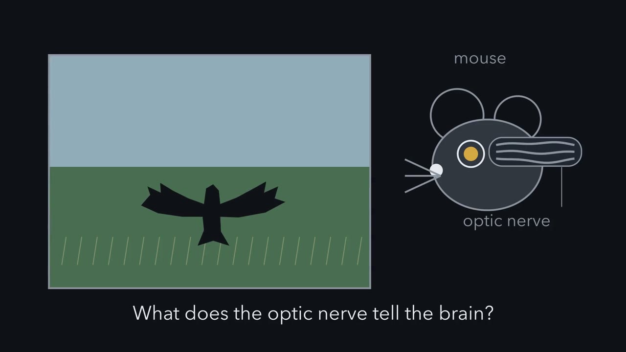 ▶ Watch Many Maps, Not One Picture · 2:08
Read the transcript of “Many Maps, Not One Picture”
Film transcript: Many Maps, Not One Picture
A hawk's shadow slides across a meadow. What does a mouse's optic nerve tell its brain about it? Every signal the brain receives from the eye leaves through ganglion cells. They are the retina's only output neurons, and their axons make the optic nerve. So does that nerve carry a picture, like a camera cable? It does not. A mouse has more than 40 types of ganglion cell. Each type reports the scene through its own filter. Some filters are simple. They signal local differences in brightness. Others are highly selective. They detect a small object moving, or motion in one direction. Bipolar and amacrine circuits inside the retina build each filter, before any spike leaves the eye.
Now look down on the retina as a flat sheet, and light up one type. Its cells spread across the retina. Each cell tends to keep some distance from its neighbours. Their dendrites can overlap a lot, and spacing and arbor size vary across the retina. That even spacing is called a mosaic. So one type draws one map of the scene. Lay a second type over the first. Then a third. Predict. If each type draws one map, what does the optic nerve carry?
More than 40 overlapping maps of the scene, each filtered differently. The brain can combine maps to build new features. But information that no map carries is gone before the brain has a chance. The same idea suggests a check. If a type is really two, its spacing usually looks less regular. And more arbors cover each point than for comparable types. These are clues, not proof. Hold one rule in mind. One type, one mosaic, one map.
From the film
- The optic nerve carries many overlapping, differently filtered maps of the scene, not one picture.
- In the mouse, each of more than 40 ganglion cell types reports the scene through its own filter, built by retinal circuits before any spike leaves the eye.
- One type, one mosaic, one map: the cells of a type usually keep their distance from one another.
A hawk’s shadow slides across a meadow. What does a mouse’s optic nerve tell its brain about it?
Not a picture. Every signal the brain receives from the eye leaves through ganglion cells, the retina’s only output neurons, whose axons make the optic nerve. A mouse has more than 40 types of ganglion cell, and each type reports the scene through its own filter. Some filters are simple: they signal local differences in brightness. Others are highly selective: they detect a small object moving, or motion in one direction. Bipolar and amacrine circuits inside the retina build each filter before any spike leaves the eye, so the visual cortex can only work with what these channels deliver. Information that no channel carries is gone before the brain has a chance, though the brain can combine channels into new features.
The retina followed the signal from photoreceptor to ganglion cell and built ON and OFF centre-surround fields; sensory coding weighed labelled lines against population codes. This lesson watches one filter at work, then asks how anyone knows that a group of cells is one real type.
One cell that ignores the world moving
Read the transcript of “The Cell That Ignores the World Moving”
Film transcript: The Cell That Ignores the World Moving
How could one cell tell a moving object from a moving world? In 2012, Zhang and colleagues recorded from W3 cells in isolated mouse retina. Start with a spot. Brighten a small spot over the cell, and it fires. Dim the same spot, and it fires again. The cell takes excitation from the ON pathway, driven when light goes up, and from the OFF pathway. So a change of either sign excites it. The two inputs add rather than cancel. Now motion. A small textured patch moves over the cell's centre, and the background stays still. The distant surround is a wide ring far outside the centre. The cell fires many spikes. Say 40. Now the whole scene moves together.
The centre gets exactly the same stimulus. Predict. If the cell listened only to its centre, what would it do now? It would fire just as much. It does not. It falls nearly silent. Say 3 spikes. So motion far out in the surround must be silencing it. Zhang and colleagues found that this happens in two places at once. Part is presynaptic. The excitation is suppressed before it reaches the cell, so less of it arrives. Part is postsynaptic. Inhibition lands on the W3 cell itself. Older work on similar cells in other species proposed wide-field amacrine cells as the source of this kind of suppression. Where does the excitation come from? Much of it does not come straight from bipolar cells.
It arrives through the VG3 amacrine cell, an excitatory amacrine cell. So the circuit that builds the selection starts before the ganglion cell sees the signal. Two amacrine cells, two jobs. VG3 brings excitation in. Wide-field cells are the proposed brake. A W3 cell answers one question. Is something small moving differently from everything else? When the eye or head turns, the whole image slides together. The authors proposed these cells as alarm neurons for overhead predators. That is a hypothesis. The experiments used isolated retina, and no behavioural test of necessity was done. A second channel is the JAM-B cell, an OFF cell. Most labelled cells had a lopsided dendritic arbor.
These lopsided cells preferred movement from the cell body toward the dendrites. The filter is built inside the retina. The scene motion this cell ignores still travels in other channels.
From the film
- A W3 cell fires for a small object moving over a still background and falls nearly silent when the whole scene moves.
- Part of that silencing is presynaptic and part is postsynaptic, and the VG3 amacrine cell supplies much of the excitation.
- The JAM-B cell is a second channel: in isolated retina, its lopsided cells preferred movement from the cell body toward the dendrites.
- Calling W3 cells alarm neurons for overhead predators is a hypothesis, because the experiments used isolated retina.
Start with a single channel and watch it work. Zhang and colleagues (2012) recorded from W3 cells in isolated mouse retina, using a mouse line, TYW3, that makes these cells fluorescent. (That line was later found to label several types; the brightly labelled local-change cell is now called W3B.)
First, a spot. A W3 cell fires when a small spot over it brightens, and fires again when the same spot dims; a plain ON cell would fire only to the brightening. The W3 cell pools excitation from both the ON pathway (driven when light goes up) and the OFF pathway (driven when light goes down). Each input is “rectified”: it drives the cell for its own sign of change and does little for the other. So the two inputs add rather than cancel, and a W3 cell is excited by local change of either sign.
Now motion. Picture a small textured patch moving over the cell’s centre. The “distant surround” in the table is a wide region far outside that centre.
| Stimulus (illustrative spike counts, not recorded data) | Centre | Distant surround | W3 spikes |
|---|---|---|---|
| Small object, still background | moving | still | many (say 40) |
| Whole scene moves together | moving | moving with it | few (say 3) |
Predict. The centre gets the same stimulus in both rows. If the W3 cell listened only to its centre, what would the second row show? What must the surround be doing?
Check your prediction
It would fire just as much. It does not, so motion far outside the centre must be silencing it. Zhang and colleagues found that motion in the distant surround acts in two places at once. Part of the silencing is presynaptic: the excitation is suppressed before it reaches the W3 cell, so less of it arrives (this lesson does not pin down at which input terminals). Part is postsynaptic: inhibition lands on the W3 cell itself. Older work in other species proposed wide-field amacrine cells, whose processes spread far across the retina, as the source of suppression by global motion.
So a W3 cell answers one question: is something small moving differently from everything else? The whole image slides together when the eye or head itself turns, so a cell like this can tell an object’s own motion from the scene sliding past. The authors proposed that W3 cells may act as alarm neurons for overhead predators. That is a hypothesis: the experiments established selectivity and circuit properties ex vivo, and no behavioural test of necessity was done.
Where the filter is built. Nothing in the photoreceptors tells object motion from scene motion; the circuit between them and the W3 cell builds the difference. Much of the W3 excitation does not come straight from bipolar cells. It arrives through an excitatory amacrine cell, the VG3 amacrine cell (Krishnaswamy and colleagues, 2015). Keep the two amacrine cells apart: the VG3 cell brings excitation in, and wide-field amacrine cells are the proposed brake. The scene motion that W3 ignores still travels in other channels.
JAM-B: a lopsided cell with a preferred direction
A second channel shows a different filter, tied to the cell’s shape. Kim and colleagues (2008) used a genetically marked mouse line (JAM-B-CreER) to label a class of OFF ganglion cells; the label was strongly enriched for the class but may not be pure. About 85% of labelled cells had markedly asymmetric dendritic arbors, and in isolated retina these asymmetric cells preferred movement from soma toward dendrites. Because the lens inverts the image, that direction on the retina corresponds to upward motion in the visual field, so a statement about preferred direction needs its frame. Symmetric labelled cells in ventral retina showed no clear preferred direction, so a type’s filter may itself change across the retina.
W3 reports local change, JAM-B prefers one direction, and other types report contrast, colour or light level.
The one idea to carry through this lesson: one type, one mosaic, one map. As a working picture, a ganglion cell type is a set of cells that share broadly the same filter on the scene and spread across the retina, usually spaced out in their own mosaic, so that together they sample the visual field. The mouse optic nerve therefore carries more than 40 overlapping maps of the scene, each filtered differently.
Read it as a working picture tested on mouse ganglion cells, not a definition. Density, arbor size and even response properties change across the retina, as W3 density and JAM-B direction preference do, and the brain need not read each map as a separate labelled line, since targets can combine channels.
Testing a type: agreement and a mosaic
Read the transcript of “One Type or Two? Four Ways to Count”
Film transcript: One Type or Two? Four Ways to Count
An analysis draws a group around some cells. Is it one type, or two? Recall the idea. A real type usually spaces its cells out in its own mosaic. Here is one type. Its cells keep their distance, and its arbors overlap. The coverage factor is the number of arbors over an average point. Now pour in a second type, placed independently. Colour every cell the same. Predict. Treated as one type, what happens to the spacing, and to the coverage?
The spacing usually turns patchy. A cell of one type can sit right beside a cell of the other. And the coverage adds up, so it reads higher than either type's own. So an unusually high coverage can be a sign that two types were merged. But some real types are only weakly regular. A mosaic is strong support, not a strict rule. Each census method tests a different part of the rule. Imaging grouped cells by light response, and found at least 32 types. RNA sequencing grouped cells by gene expression, and ended with 46. One cluster held two direction-selective types already known from function. Clustering alone had missed them. Another team recorded spikes and found 42 functional types.
For some cells, they also read that same cell's RNA or shape. There, three sustained ON direction-selective types shared one RNA cluster, called C10. Electron microscopy of one small patch supported at least 35 types. These are not rival answers. Each reflects a method, a preparation and a resolution. The most trustworthy types are the ones that more than one method finds. A primate needs its own census. In the macaque fovea, one red or green sensitive cone feeds its own midget bipolar cells. That private centre keeps fine spatial detail. Midget clusters made up about 85% % of sampled foveal ganglion cells. Shared ancestry with mouse cells does not mean a shared size, frequency or job.
Combine the evidence. A separate mosaic strengthens the case for a type, but it is not required.
From the film
- A real type usually spaces its cells out in its own mosaic, so merging two types usually makes spacing patchy and coverage higher.
- A mosaic is strong support for a type, not a strict rule, because some real types are only weakly regular.
- Imaging, RNA sequencing, spike recording and electron microscopy gave different counts because each reflects a method, a preparation and a resolution, not rival answers.
- The macaque fovea needs its own census, since midget clusters made up about 85% of sampled foveal ganglion cells.
Calling W3 or JAM-B a channel assumes that its cells form one real type. Three kinds of evidence can define a ganglion cell type:
- A functional type is a group of cells with the same light response.
- An anatomical type shares a dendritic shape and the depth in the inner plexiform layer (IPL, where bipolar, amacrine and ganglion cell processes meet) at which that shape sits.
- A molecular type shares an expression profile. A cluster is different: it is the group an algorithm draws around such profiles, and it may hold one type or several.
The usual standard for calling a group a type asks for agreement among them, plus a mosaic: cells of the type are spaced regularly across the retina. A mosaic describes the spacing of cell bodies; the dendrites of one type can still overlap a lot.
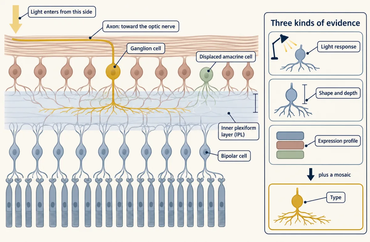
The sensory neuron atlas met the same problem in the dorsal root ganglion, and the answer is the same here: a transcriptomic or anatomical cluster becomes a type when response, shape and expression are tied to one another and, ideally, when genetic access lets you label or manipulate it.
Coverage: how a type samples the scene
A useful measure of how a type samples the field is the coverage factor, the average number of dendritic arbors that cover a retinal location. A value above 1 is normal, because the arbors of one type overlap.
coverage factor = cell density (cells/mm²) × mean dendritic field area (mm²)
Predict. The one idea suggests a check on whether a group is one type. Suppose an RNA cluster secretly holds two types, each with its own regular mosaic placed independently of the other, and you treat the cluster as one type. What happens to its spacing? What happens to its coverage factor?
Check your prediction
The spacing usually becomes less regular. Each type keeps its own cells apart, but nothing stops a cell of one type from sitting right beside a cell of the other, so the merged group has some very short neighbour distances. The coverage adds up: the merged density is the sum of the two densities, so the coverage factor comes out higher than either type’s own, and twice as high if the two types match in density and arbor size. Bae and colleagues (2018) warned that coverage alone can mislead, but an unusually high coverage factor can be a sign that two types have been merged. Neither sign proves a merge, since some real types are only weakly regular and some have high coverage, so the next step is to look for differences in response, shape or expression.
Worked problem, coverage. Zhang and colleagues (2012) reported, for W3 cells in mouse retina, a peak density of 440 cells/mm² in ventral retina and a mean dendritic field area of 10,300 µm². Step 1: convert units. 10,300 µm² × 10⁻⁶ mm²/µm² = 0.0103 mm². Step 2: multiply. 440 cells/mm² × 0.0103 mm² = 4.53. About 4.5 arbors cover an average point.
Predict. Does a coverage of about 4.5 show that the W3 count mixed several types together?
Check your prediction
Not by itself: a value above 1 is normal for one type. The figure also pairs a regional peak density with a mean area, so treat it as an estimate. And because TYW3 labels several types, if the density counted more than one of them, the density, and so the coverage, may be overestimated for W3B.
- Unit conversion
- 10,300 µm² × 10⁻⁶ = 0.0103 mm²
- Coverage factor, expected (density × area)
- 440 × 0.0103 = 4.53
- Mean count at the probe points, in this draw
- 4.5
- Cell bodies in the patch, in this draw (expected)
- 27 (27.5)
- Band from the spread
In this sketch: circular dendritic fields of equal size, uniform density inside the patch, cell positions on a jittered mosaic (the jitter amount is arbitrary) drawn at random (cells just outside the edge also cover points inside it), and a point counts as covered if it lies inside an arbor. The patch is 0.25 mm on a side and not to scale for any real field.
Coverage factor = cell density × mean dendritic field area, with µm² converted to mm² (× 10⁻⁶); it is an average number of arbors per location, so it is only as good as the density and area you put in.
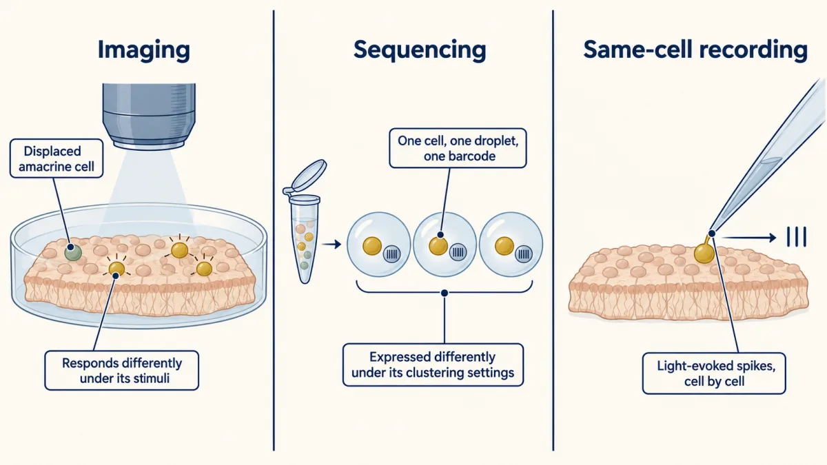
Four ways to count
Recall the one idea: a real type shares one filter and, usually, its own mosaic. Each census method tests a different part of that claim, by one kind of evidence, so each gives its own number.
| Method | Groups cells by | Result | Study |
|---|---|---|---|
| Two-photon calcium imaging of the ganglion cell layer | light-response profile | at least 32 functional types | Baden and colleagues, 2016 |
| Droplet single-cell RNA sequencing | gene expression | 46 types (45 clusters, one split) | Tran and colleagues, 2019 |
| Same-cell recording, with RNA or shape from subsets | spike response, checked against RNA and shape | 42 functional types | Goetz and colleagues, 2022 |
| Electron microscopy of a patch whose light responses were imaged | arbor shape and IPL depth | 47 anatomical clusters, at least 35 types | Bae and colleagues, 2018 |
Imaging sees what responds differently under its stimuli, and the imaged layer also holds displaced amacrine cells, interneurons that had to be set aside before counting. Sequencing sees what is expressed differently under its clustering settings. Same-cell recording ties a response to RNA or shape within one cell. Anatomy sees shape exactly, but only in one small patch. Bae and colleagues drew 47 anatomical clusters. The clusters that held up to internal validation, together with types already securely known, gave a lower bound of 35 types. So 47 counts clusters, and 35 is a floor on types. Two of the four results are lower bounds, and the authors read the studies as converging on about 45 types. So the four numbers are not rival answers to one question. Each reflects a method, a preparation and a resolution, and the most trustworthy types are the ones that more than one method finds.
Predict. Tran and colleagues’ RNA clustering (droplet single-cell RNA sequencing, uninjured adult mice) gave 45 clusters. One of them held two direction-selective types already known from function, ON-OFF cells preferring ventral or dorsal motion, which no marker had separated. What does that tell you about a type count from clustering alone?
Check your prediction
Clustering alone can miss real types. The authors split that cluster with a semi-supervised analysis, giving 46 types, so the count depends on prior knowledge as well as on the data.
The same-cell census found a second mismatch of this kind. Goetz and colleagues recorded spikes from all the cells they sampled and, in subsets, collected the same cell for RNA (a Patch-seq variant) or recovered its morphology. Because response and RNA came from one cell, the alignment showed that the map between function and RNA is not always one to one: three sustained ON direction-selective types, which differ in preferred direction, aligned with a single cluster, C10.
Mouse is not macaque: the primate fovea
Which types a retina has, and in what shares, differs between species. The retina of humans and macaques has a fovea, which a mouse retina lacks. The fovea packs cones and midget ganglion cells densely. There each red- or green-sensitive (L or M) cone feeds its own ON and OFF midget bipolar cells, which connect one to one with ON and OFF midget ganglion cells.
Predict. In this private line, the centre of a midget cell’s receptive field takes its signal from one cone, not from a pooled group. What does that preserve for the brain?
Check your prediction
The fine spatial detail of the cone array. That is why midget cells support high-acuity vision. Their surround still pools neighbouring cones, and in the fovea midget cells also carry red-green colour signals. Parasol cells respond transiently and are sensitive to motion and to low contrast, functionally like the transient alpha cells of rodents.
Peng and colleagues (2019) profiled cells from the fovea and the periphery of adult macaques, and checked the identities of the midget and parasol clusters with fluorescent in situ hybridization and viral labelling of cell shape. Midget clusters accounted for about 85% of sampled foveal ganglion cells and parasol clusters for 11%. When the group compared macaque and mouse, bipolar and amacrine types matched closely, but ganglion cell types diverged, and midget and parasol cells were taken to be primate specialities. A later atlas of 17 species (Hahn and colleagues, 2023) found their mouse counterparts.
Midget cells correspond to sustained alpha cells, which make up about 2% of mouse ganglion cells, and parasol cells to transient alpha cells. One of the mouse sustained alpha cells, the sustained ON alpha cell, is the M4 cell of melanopsin cells. ON direction-selective cells and melanopsin cells are also conserved. A shared ancestry does not mean a shared size, frequency or job.
Worked problem, composition. In the foveal sample, midget plus parasol is 85% + 11% = 96%, leaving about 4% for every other cluster. In a made-up sample of 5,000 foveal cells that would be 0.04 × 5,000 = 200 cells. The 4% says how much of the sample is left over, not how many types share it.
The percentages are of sampled cells from the macaque fovea; they are not whole-retina figures and not human frequencies, and a mouse type cannot be renamed as a human type because the names look alike. The mouse census is a map of a mouse, and a primate needs its own.
Where next: how the direction-selective circuits are built is the subject of the next lesson, non-image-forming channels appear in melanopsin cells, and photoreceptor adaptation and degeneration asks what changes when the input fails. Developmental lessons on spontaneous activity and topographic maps cover how the output layer is wired, and microscopy and images covers the reconstruction methods.
Design problem
Return to the three Goetz types that share cluster C10. Does the retina send three direction channels here, or one type with several response modes? Given responses for all the cells and RNA or shape for subsets, say what each measurement can decide, and propose what to add.
Saved in this browser only.
One way to do it
Start with what each measurement is. A cluster is separable expression, and its number depends on sequencing depth and clustering settings. A functional type is a shared response, and a separate mosaic is independent evidence for it, so sharing one cluster does not make the three the same.
The data as given support three functional types that RNA does not separate at this resolution, as happened with two direction-selective types in the Tran atlas. Goetz and colleagues separated them by preferred direction, as is usual for direction-selective cells, and treat them as three types.
A better experiment avoids comparing data sets and extends the same-cell approach. Record the light response of many more cells in each class, then recover RNA and shape from those same cells. If the three response classes still share their expression, test whether each one has its own mosaic, with its own regular spacing and coverage. Ask for genetic access to one of the three, say a driver line that labels one class, so the class can be marked and manipulated. If a finer clustering later splits C10 into three along function, that supports three types. If the three classes together form one regular mosaic and none forms its own, that points toward one type with several response modes, though spatial tests alone cannot settle it.
Going deeper
The study details behind the main line (who measured what, in which animals, with how many cells) and side results it leaves out.
The three functional and molecular censuses
Imaging. Baden and colleagues imaged isolated ventral retina from mice aged four to eight weeks, using two-photon calcium imaging of the ganglion cell layer. The data set held 11,210 cells, not 11,210 ganglion cells: 14 groups of displaced amacrine cells were separated from the ganglion cell groups before counting. The study distinguished a minimum of 32 functional types, four of them from clusters the authors labelled uncertain, and concluded that some unusually abundant types probably hide further subdivisions. The imaging was acquired at 7.8 Hz, so it follows a response profile, not individual spikes.
Sequencing. In droplet sequencing each dissociated cell is captured in its own droplet with a barcode. Tran and colleagues profiled 35,699 high-quality ganglion cell transcriptomes from mice at postnatal day 56, flow-sorted from uninjured retina. Types ranged from 0.15% to 8.4% of the cells profiled, and most clusters needed a combination of two marker genes for a unique identity. These are shares of flow-sorted, dissociated cells, which need not match the true frequencies of the types in the retina.
Worked problem, rare types. How many cells does a 0.15% type contribute? 0.0015 × 35,699 = 53.5, so about 54 cells. The largest type, 8.4%, gives 0.084 × 35,699 = 2,998.7, about 3,000 cells. The smallest type therefore rests on roughly fifty cells, and a different depth or clustering setting could merge it or split it. A type this rare is also hard to test for a mosaic, since a small patch of retina may hold few of its cells.
Same-cell recording. Goetz and colleagues recorded light-evoked spikes in the cell-attached configuration from 1,859 ganglion cells in isolated retina from mice 4 to 12 weeks old. They estimated that their 42 types matched 89% of the types in the Eyewire anatomical catalogue (Bae 2018), which is a share of types, not of all ganglion cells.
Dense reconstruction and the anatomical count
Helmstaedter and colleagues (2013) used serial block-face electron microscopy, in which the face of a tissue block is imaged and shaved away repeatedly, with manual tracing and machine-learning segmentation, to reconstruct 950 neurons and their mutual contacts in the mouse IPL. The authors cautioned that not all contacts are synapses, so a contact map proposes partners and does not prove them.
Bae and colleagues (2018) worked in one ex vivo mouse retinal patch, called e2198, in which light responses had been imaged and the same tissue then imaged by electron microscopy, so each reconstructed arbor could be set beside its own response. They extracted calcium signals for 326 cells and kept 381 reconstructed ganglion cell arbors, which formed the 47 anatomical clusters.
Density conservation
The density-conservation hypothesis says that the aggregate dendritic density of a type (its total dendrite per unit area of retina) should be about uniform across the retina, even though cell density and arbor size vary across the retina. The coverage factor in the main line is a related measure that counts arbors and not total dendrite. Bae and colleagues (2018) proposed density conservation to replace the older demand that a type’s arbors tile with little overlap.
Inside the W3 circuit: amacrine diversity and layer depth
Amacrine cells are themselves diverse. Yan and colleagues (2020) sequenced 32,523 amacrine cells from mice at postnatal days 18 to 19 and reached 63 putative amacrine types, which they treated as a lower limit, so this repertoire is part of the circuit behind each channel.
Where a ganglion cell’s dendrites sit in the IPL helps set which inputs it receives: in one reconstructed patch, cells arborising in the inner margin of the IPL had on average more sustained responses.
W3 and JAM-B: labelling, history and colour
W3 arbor size. The mean dendritic field area in the coverage problem was 10,300 ± 500 µm² (n = 25).
Earlier object-motion cells. Older recordings in isolated salamander and rabbit retina (Ölveczky, Baccus and Meister, 2003) had already found a subset of ganglion cells that preferred differential motion of centre and surround, and proposed wide-field amacrine cells as the source of suppression by global motion. Zhang’s group concluded that W3 corresponds to the rabbit local edge detector, which does not make every object-motion cell in every species a W3 cell.
JAM-B labelling. CreER is a recombinase switched on by tamoxifen, so a reporter then labels cells that expressed the marker. A few hundred ganglion cells per retina were marked, at least 90% of them expressing JAM-B.
JAM-B colour. Later work found that JAM-B cells also report a UV-green colour contrast.
Where the channels go
Anterograde tracing shows that mouse ganglion cells reach more than 50 areas of the brain, but maps of which type goes to which area are still rudimentary.
Abundance is not importance
A type’s share of the census says little about its job. Melanopsin cells are sparse, yet they are crucial for circadian entrainment and the pupillary light reflex.
The macaque sample
Peng and colleagues profiled approximately 165,000 cells from adult male macaques (Macaca fascicularis, aged three to nine years), and found 16 foveal and 18 peripheral ganglion cell clusters.
Your notes
Select any text in the lesson to highlight it or add a note to it. Your highlights and notes are saved in this browser and collected in your notebook.
This browser is not letting the site save anything (a private window or strict privacy settings), so highlights and notes will be lost when you leave the page.
How we measure it
Two-photon calcium imaging of the ganglion cell layer
A fluorescent calcium indicator reports activity in many cells at once while light stimuli are shown to an isolated retina. Cells are then grouped by response, which gives a functional census but includes displaced amacrine cells that must be sorted out.
Droplet single-cell RNA sequencing
Each dissociated cell is captured in its own droplet with a barcode, so thousands of transcriptomes can be read and clustered. It separates cells by expression but does not by itself say what they compute.
Patch-seq
A cell's light response is recorded with a pipette, and the same cell is then collected for RNA sequencing, with morphology in some cases. The response and the transcriptome belong to one cell, so the response and the transcriptome need no matching to each other, though placing the cell in a reference atlas still does.
Serial block-face electron microscopy
A tissue block is imaged and a thin layer removed, over and over, giving a stack from which neurites can be traced. It gives exact shapes and contacts, but only for a small fixed piece of tissue.
Practice questions on this lesson (3) → MCAT-style, original, each with an explanation
Where this lesson fits
Before thisReview first
- Sensory Neurons by Their Genes: the Atlas EraThis course · Lesson 3
It shows how gene-expression clusters become real neuron types, the same question asked here for ganglion cells.
- Five Ways to Turn a Stimulus into a CurrentThis course · Lesson 1
You need to know how photoreceptors turn light into a current before asking what ganglion cell filters do with that signal.
After thisStudy next
- Computing Motion in the RetinaThis course · Lesson 19
It shows how retinal circuits build the direction-preferring channel previewed here with JAM-B and the direction-selective types.
- Melanopsin Cells: Light for the Clock and the PupilThis course · Lesson 20
Melanopsin cells are a sparse ganglion cell type whose clock and pupil job shows abundance is not importance.
- Calcium Feedback Sets Photoreceptor Gain, and When Photoreceptors DieThis course · Lesson 21
It asks what happens to these ganglion cell channels when photoreceptor input changes or fails.
Suggested by an AI model from the lessons themselves, then checked. How we use AI
Finish line
Test yourself
9 questions
Practice and MCAT-style, with explained answers.
Next · Lesson 19
Computing Motion in the Retina
A cell in the eye fires to a spot moving left and stays quiet for the same spot moving right. Which neuron makes the difference?
Continue →← Lesson 17 · Sensing the Gut: Enteroendocrine Cells and Nutrient Signals