Neuroscience · Unit 3: Sensory systems
Principles of Sensory Coding
Rewritten on : new text, figures, flashcards and film. Your notes and highlights stay, but the text around them may have moved.
A heavier weight on a frog's muscle receptor did not make bigger impulses, only more of them. How do identical spikes carry a whole world?
Pause when the reading reaches a film, and offer to play it. Saved on this device.
Watch the film now, or keep listening
Builds on:The Resting Membrane and Passive SignalsThe Action Potential and ConductionIntegration, Inhibition and NeuromodulationWhy these?
 ▶ Watch What a Spike Means · 2:43
Read the transcript of “What a Spike Means”
Film transcript: What a Spike Means
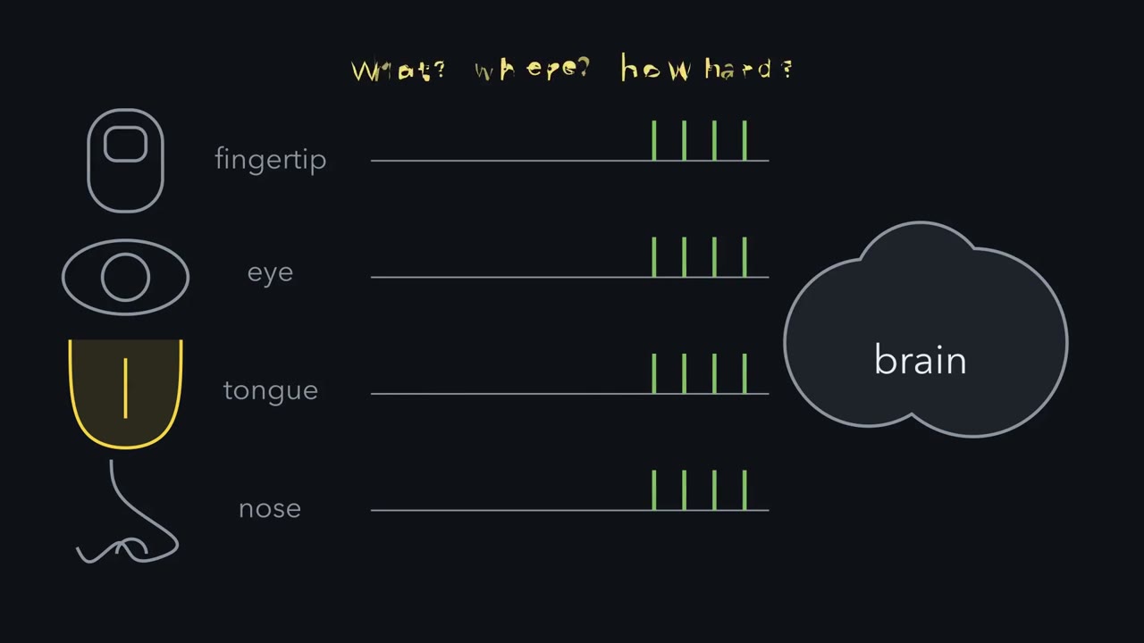
Every sense ends in the same currency: spikes that look alike. So how does a spike say what touched you, where, and how hard? In 1926, Edgar Adrian and Yngve Zotterman recorded one stretch receptor in a frog muscle. Then they hung weights on the muscle. A heavier weight stretches the receptor more. Will its spikes get bigger, or will they come more often?
They come more often. Every spike stays the same size. And while a weight is held, the firing slowly falls. So the rate tells you how much. Now the what. Pressure on the closed eye is seen as light. Activity in the optic nerve means light, whatever started it. So the kind of sense comes from the line. Whether every quality works this way is still argued. A tuning curve plots a neuron's mean firing rate against one feature of the stimulus. The count varies from trial to trial. That spread is noise. Here is the one idea, for spikes counted over a fixed time. On each trial, a neuron's rate is its tuning curve, read at the stimulus, plus a fluctuation that averages to zero.
Which neurons respond, and their relative firing rates, together tell you what, where and how much. A small change is easiest to see where the rate changes a lot, compared with the noise. Spike timing can carry information too. How is the rate set? In touch, force opens channels, mostly in the nerve ending itself. In a simple model, each open channel pulls the balance point toward 0 mV. So the receptor potential is graded. Each extra channel moves it less, as the voltage nears 0 mV.
But a graded potential fades as it spreads. To reach the spinal cord, it must become spikes, which regenerate. Receptive fields help tell you where. Many afferents used for fine touch have small fields on a fingertip and larger ones elsewhere. Field size also depends on receptor type. Endings are tuned in time, too. Rapidly adapting endings report change. Slowly adapting endings keep firing, and report the stimulus itself. So a spike means what its neuron is tuned to. Next, neighbours compare.
From the film
- A spike means what its neuron is tuned to.
- For spikes counted over a fixed time, a neuron's rate is its tuning curve read at the stimulus plus a fluctuation that averages to zero.
- Which neurons fire and their relative rates together tell you what, where and how much; in Adrian's frog stretch receptor, heavier loads made spikes more frequent, not bigger.
- A graded receptor potential fades as it spreads, so it must become spikes to reach the spinal cord or brain.
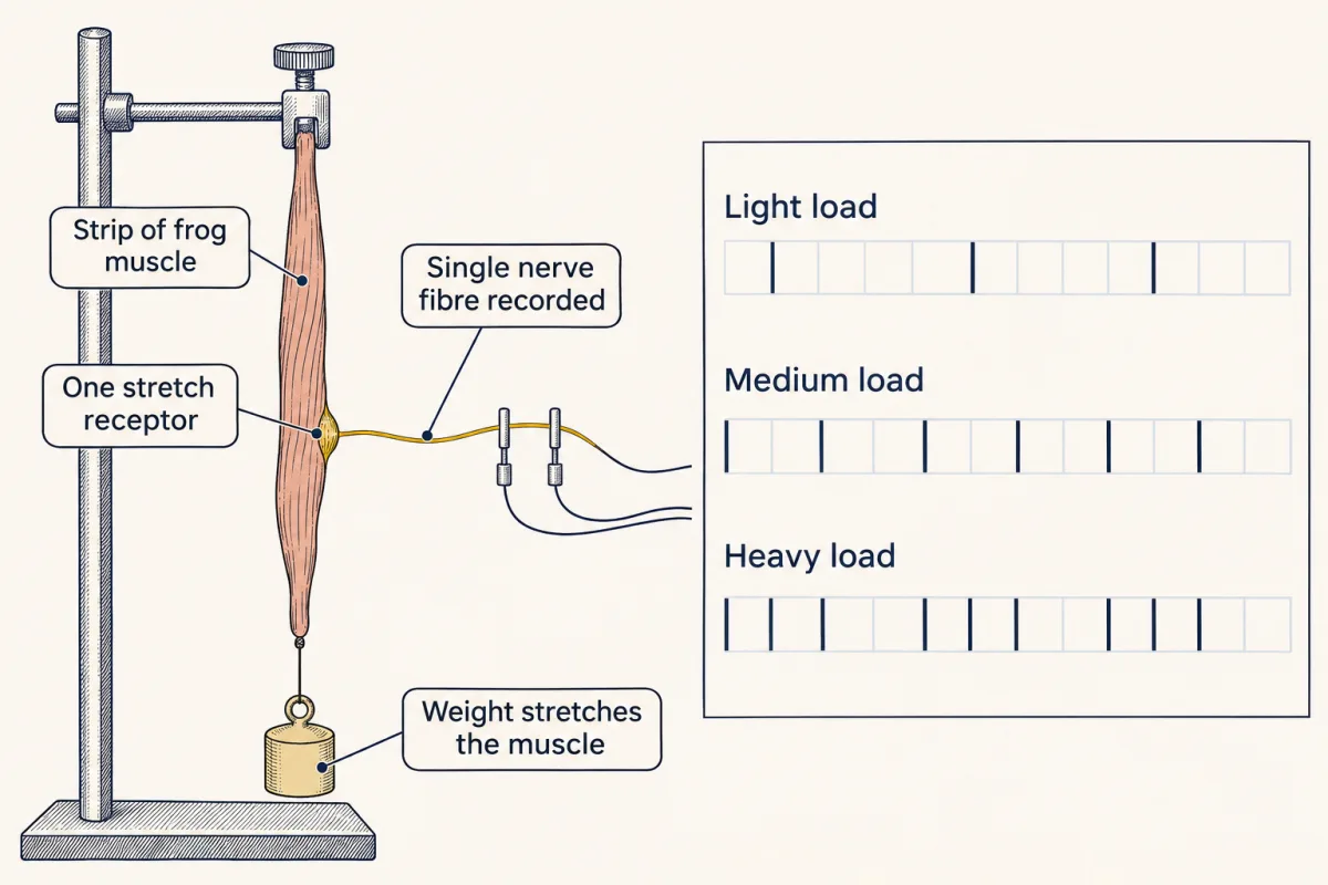
In 1926 Edgar Adrian and Yngve Zotterman cut a frog muscle down until one stretch receptor was left, hung weights on it, and recorded what that single ending sent along its nerve fibre.
Every sense you have ends in the same currency. A fingertip ending, a rod in the retina, a taste cell and an olfactory neuron all produce graded voltages. The afferent neurons, which carry signals toward the brain, send trains of spikes that look alike. So how does a train of identical spikes say what touched you, where, and how hard?
One ending, three weights
In the 1920s no one could yet say what a single sensory ending sent to the brain, because a whole nerve mixes the activity of many fibres. Adrian and Zotterman kept cutting strips from the muscle until the record showed a single, regular series of impulses, their sign of one active ending.
Predict. A heavier weight stretches the receptor more. Will its impulses get bigger, come more often, or both?
Check your prediction
They come more often, and they do not get bigger. Picture the record: three loads, three trains of impulses, every impulse the same height, sitting closer together under the heavier load. While a load is held, the frequency slowly falls. These two facts, rate coding and adaptation, are still the first two taught about sensory coding.
If every spike looks alike, the record raises four puzzles.
- What. How does the brain know a signal came from touch and not from light?
- Where. How does it know which patch of skin was touched?
- How much. How does it read the strength of the stimulus?
- How fine. How can it detect a change so small that it barely moves the firing rate?
What a spike means
Adrian’s record answers the third puzzle. In his single fibre, heavier loads did not make the spikes bigger: stimulus strength was carried by their frequency, so how often spikes come tells you how much. A stronger stimulus also recruits more afferents, so the number of active fibres carries intensity too.
The first puzzle has a different answer: which fibre is firing tells you what. In a labelled line, a fibre’s activity means one thing, say “sweet”, however it was activated. The classic example, behind Müller’s law of specific nerve energies, is that pressure on the closed eye is seen as light. The pressure is not light, but activity in the optic nerve means light to the brain, whatever started it. Whether every quality of every sense runs on dedicated lines is still argued (see the end of the lesson).
To put “which” and “how much” into one rule, you need two terms. A neuron’s tuning curve plots its mean firing rate against one property of the stimulus, such as the orientation of a bar or the frequency of a tone. Present the same stimulus many times and the spike count in a fixed time window fluctuates from trial to trial. The standard deviation of that fluctuation is the neuron’s noise.
The one idea to carry through this lesson. A spike means nothing by itself. It means what its neuron is tuned to.
- Count a sensory neuron’s spikes over a fixed stretch of time. On each trial its firing rate is its tuning curve read at the stimulus, plus a fluctuation that averages to zero: rate = tuning curve(stimulus) + fluctuation.
- Which neurons fire and their relative rates together tell you what, where and how much.
- For otherwise similar responses, a small change is easiest to detect where it moves the mean rate a lot compared with the noise.
The rule has two limits. Some senses also carry information in spike timing, such as the latency of the first spike in touch and phase locking to the sound wave in hearing. And the rule says what information a neuron carries, not how the brain reads it out.
From stimulus to rate
Transduction is the conversion of a stimulus into an electrical signal at a sensory receptor. The first signal is the receptor potential, a change in membrane voltage whose size grows with stimulus strength.
The machinery differs by sense. In touch, force opens mechanically activated channels, mostly in the ending of the sensory neuron itself (Merkel cells, skin cells that contact some touch endings, also transduce; see Going deeper). Removing the channel Piezo2 from adult mouse sensory neurons and Merkel cells removed much of touch (Ranade and colleagues, Nature, 2014). Vertebrate photoreceptors use a receptor protein and a cGMP cascade, and light hyperpolarizes them, making the inside more negative. Smell, and sweet, umami and bitter taste, also use receptor proteins, while sour taste and one pathway for salt work through ion channels (see Going deeper). The cascades belong to senses and cGMP; here we follow what the voltage does next.
Why the receptor potential is graded
Use the rule from the action potential: with no current injected, the voltage moves toward a balance point, the average of the equilibrium potentials weighted by their conductances, and settles there. Take a simple passive model: the resting membrane’s channels, which together reverse at −65 mV, plus transduction channels, cation channels whose current reverses near 0 mV. With two kinds of channel, the balance point is
Vm = (grest × −65 mV + gtrans × 0 mV) ÷ (grest + gtrans)
where grest is the resting conductance and gtrans the transduction conductance. Check the ends: with no transduction channels open (gtrans = 0) it gives −65 mV; with gtrans huge it approaches 0 mV.
- Each extra open transduction channel pulls the balance point toward 0 mV. A stronger stimulus opens more channels, so the voltage moves further. The response is graded.
- Put numbers on it (made-up units). With grest = 1 and gtrans = 1, the balance point is (1 × −65 + 1 × 0) ÷ (1 + 1) = −32.5 mV. Raise the transduction conductance to 2, 3 and 4 and it moves to about −22, −16 and −13 mV. Each equal increase moves it less, by about 11, 5 and 3 mV, because the voltage can approach 0 mV but never pass it. The response saturates. The model shows only this driving-force limit; real receptors also have channel kinetics, adaptation and voltage-gated currents.
- In a rod, cGMP-gated cation channels are open in the dark, and light closes them. That moves the balance point the other way, which is why light hyperpolarizes the rod.
Why it must become spikes
Like the synaptic potentials in integration and inhibition, the receptor potential spreads passively, as in the resting membrane. A passive potential fades as it spreads, over about a length constant. To travel to the spinal cord or brain, it must be turned into spikes, which regenerate along the way.
There are two routes.
- The ending is part of the afferent neuron, as in most touch. The receptor potential depolarizes the spike-initiating zone, where the axon’s spikes start, and the larger it is, the faster the neuron fires action potentials.
- The receptor is a separate cell. It changes transmitter release instead. Taste cells release onto the afferent fibres. Photoreceptors release onto bipolar cells, and the retinal circuit passes the signal on to retinal ganglion cells, whose spikes leave the eye. The rods do not drive the ganglion cells directly.
Either way, intensity reaches the brain mostly as a firing rate, which is what Adrian and Zotterman saw.
Where and when: receptive fields and adaptation
Which neuron fires also tells you where. A receptive field is the region of the sensory surface, a patch of skin or of the visual field, where a stimulus can change a given cell’s activity.
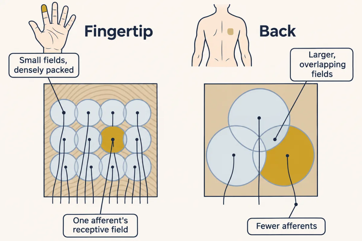
Many fingertip afferents, such as those contacting Merkel cells, have small receptive fields. Afferents of the same kind on the back have much larger ones. Receptor type matters too: a Pacinian afferent’s field can cover much of the hand.
Predict. Two blunt points touch the skin a short distance apart. Where are you more likely to feel two points rather than one: on a fingertip or on the back?
Check your prediction
On the fingertip, for two reasons. Its receptive fields are small, so two nearby points can fall in different afferents’ fields and drive different lines. And the fingertip has many more afferents per square millimetre. On the back, afferents are sparser and their fields larger and overlapping, so the spatial picture is coarser and two nearby points are harder to resolve. Firing can still differ between one point and two, and the classic two-point test can also be passed using intensity and other non-spatial cues (Tong, Mao and Goldreich, 2013).
Neurons are tuned in time as well as in space. Rapidly adapting endings fire at the start of a maintained stimulus and then fall quiet; many fire again when it is removed. They are tuned to change: a Pacinian corpuscle in the skin signals vibration. Slowly adapting endings keep firing for as long as the stimulus lasts, as Merkel-cell afferents do during steady indentation (there the Merkel cell, a separate receptor cell, helps sustain the firing), so they report the stimulus itself. Adaptation as a general circuit motif is taken up in signaling circuits.
Neighbours compare: lateral inhibition
Read the transcript of “Neighbours Compare”
Film transcript: Neighbours Compare
Each receptor reports on its own patch. So how does the eye mark an edge? Neighbours compare. The horseshoe crab, Limulus, has a compound eye. Each unit, an ommatidium, sends its own fibre into the optic nerve. Hartline, Wagner and Ratliff recorded one ommatidium. Steady light gave a steady discharge. Then they lit its neighbours as well. The discharge fell.
Was that the circuit at work? Or just stray light inside the eye? They cut the lateral connections to the recorded unit. The neighbours' light no longer inhibited it. The inhibition ran through connections between units. Think of each unit as reporting its own light, minus a share of its neighbours' light. Now take a row of units at an edge, dim on the left and bright on the right. The row continues beyond both ends. The numbers stay on screen. Deep inside each uniform region, every unit is inhibited by neighbours just like itself. Both plateaus drop. Now the dim unit right beside the edge. One of its neighbours is bright. Will it sit above its plateau, or below?
Below. Its bright neighbour inhibits it more. And the bright unit at the edge sits above its plateau, because one neighbour is dim. What changed? The step across the edge is the same size as the input step. But the uniform regions now differ less. So the edge stands out against them.
The full model of the crab eye uses each neighbour's output, and the result still holds. In the vertebrate retina, other cells build the surround. Lateral inhibition discounts uniform regions, so differences stand out. Neighbours compare.
From the film
- In the Limulus eye, lighting a unit's neighbours lowered its discharge, and cutting the lateral connections removed that inhibition.
- In a simple model, each unit reports its own light minus a share of its neighbours' light.
- Lateral inhibition discounts uniform regions, so an edge stands out against them.
So far each neuron reports on its own patch. Neighbouring receptors can also compare their inputs, and the comparison needs only subtraction.
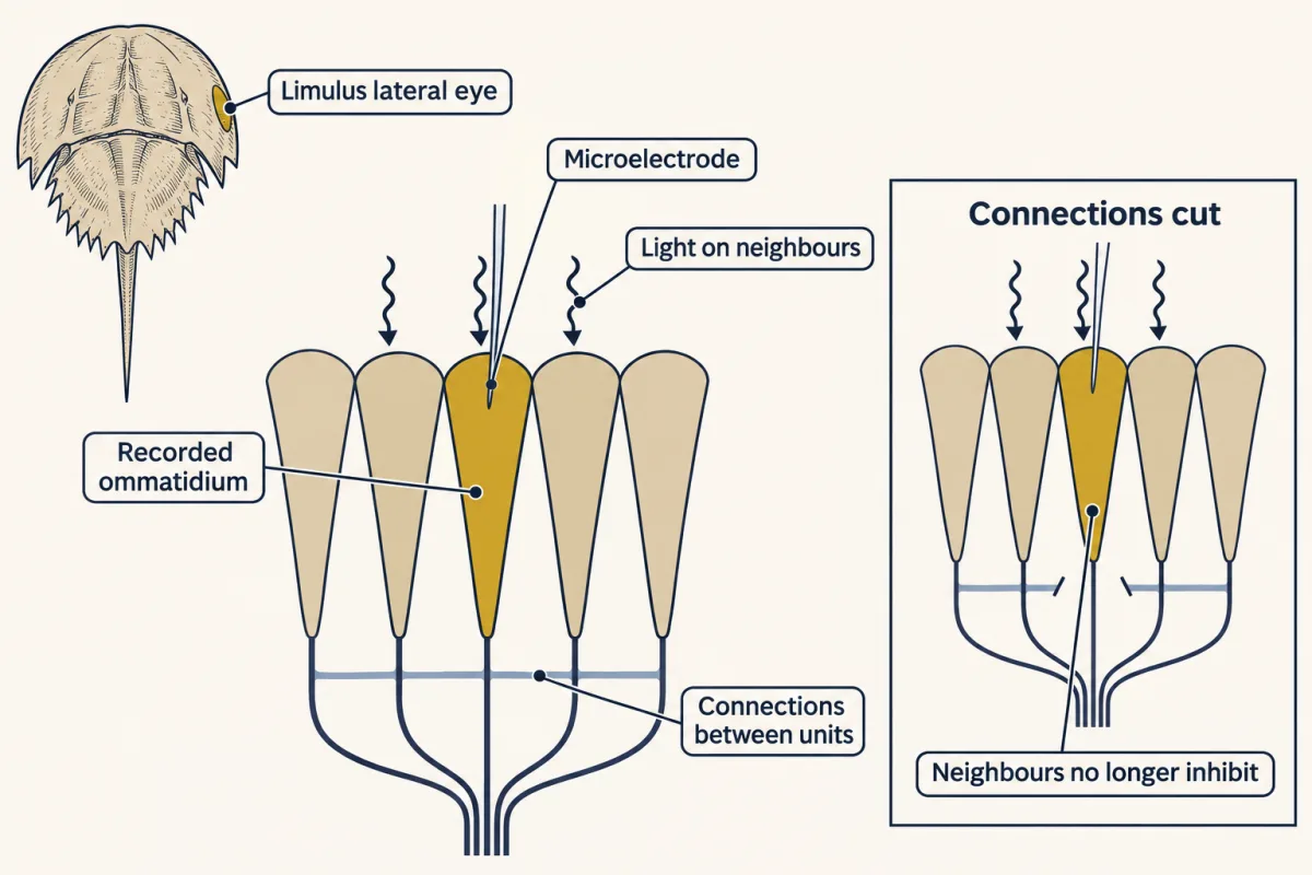
The evidence comes from the lateral eye of the horseshoe crab Limulus, a compound eye of ommatidia, each sending its own fibre into the optic nerve. Hartline, Wagner and Ratliff (Journal of General Physiology, 1956) recorded with a microelectrode inside one ommatidium, and also from single fibres dissected from the optic nerve. Picture the record.
- Steady light on the ommatidium gives a steady discharge.
- Light its neighbours as well, and the discharge falls.
- That could have been stray light or optics. So they cut the lateral connections to the recorded ommatidium, and the neighbours’ light no longer inhibited it.
The inhibition ran through connections among the units, and it exaggerated the difference in response between brightly and dimly lit regions of the eye. Think of each unit as reporting its own light minus a share of its neighbours’.
In words A unit’s output is its own excitation, minus one fifth of the excitation its two neighbours receive.
- output“output”
- what the unit sends on (made-up units)
- own excitation“own excitation”
- how strongly the unit’s own light drives it
- 0.2“point two”
- the inhibition weight: each neighbour takes away 0.2 of its own excitation. It is a chosen value for this simple model.
- left neighbour“left neighbour”
- the excitation of the unit to the left
- right neighbour“right neighbour”
- the excitation of the unit to the right
Sanity check If the neighbours are dark (zero), nothing is subtracted and the output equals the unit’s own excitation. The brighter the neighbours, the more is taken away.
Try one number
Try a uniform patch where every unit, and so both neighbours, has the same excitation, call it L.
Output = L − 0.2 × (L + L) = L − 0.4 × L = 0.6 × L.
So any evenly lit region reports 60% of its input: an input of 10 gives 6 and an input of 20 gives 12. Uniform regions are turned down by the same fraction everywhere.
Worked problem, an edge. Six receptors in a row receive excitation 10, 10, 10, 20, 20, 20 (made-up units), and the row continues beyond both ends. Apply the rule to each unit.
Interior dim: 10 − 0.2 × (10 + 10) = 6.
Interior bright: 20 − 0.2 × (20 + 20) = 12.
Predict. Now the dim unit right at the edge, which has one bright neighbour. Will its output be above or below the dim plateau of 6? What about the bright unit at the edge?
Check your prediction
Dim at the edge: 10 − 0.2 × (10 + 20) = 4, below its plateau.
Bright at the edge: 20 − 0.2 × (10 + 20) = 14, above its plateau of 12.
The dim unit beside the edge gets extra inhibition from its bright neighbour. The bright unit beside the edge gets less, because one of its neighbours is dim.
Now compare input and output. Across the edge, the output still steps by 10 (14 against 4), the same as the input step. What shrank are the uniform regions: the two plateaus now differ by 6 (12 against 6), not 10. So lateral inhibition discounts uniform regions, and the edge stands out against them.
Contrast, (bright − dim) ÷ (bright + dim), puts a number on standing out. It is 0 when the two sides are equal and approaches 1 when the dim side is near zero.
- Input: (20 − 10) ÷ (20 + 10) = 10 ÷ 30 = 0.33.
- Output plateaus: (12 − 6) ÷ (12 + 6) = 6 ÷ 18 = 0.33.
- Across the edge: (14 − 4) ÷ (14 + 4) = 10 ÷ 18 = 0.56.
The step at the edge keeps its size while the levels around it fall, so its contrast rises.
This rule is a feedforward simplification. The Hartline-Ratliff model of the real eye uses each neighbour’s output, not its input, and has thresholds; the result still holds (numbers in Going deeper). The model predicts bands at a step. People see the light and dark Mach bands mainly where a luminance ramp meets a plateau, and an abrupt step does not ordinarily show them, so the band pattern here is an analogy, and lateral inhibition is thought to be part of that story, not all of it. Limulus is not the vertebrate retina, whose surrounds are built by other cells; see the retina.
- Interior dim
- 6
- Dim at the edge
- 4
- Bright at the edge
- 14
- Interior bright
- 12
- Plateau difference (interior bright − interior dim)
- 6
- Across-edge difference (bright edge − dim edge)
- 10
In this sketch: k and the bright level are made-up values (the lesson uses k = 0.2, bright 20); each output = own excitation − k × (left + right neighbour), computed from the inputs (feedforward), no thresholds, row continuing past both ends, made-up units. Not the vertebrate retina.
This sketch is a feedforward simplification of the recurrent Hartline–Ratliff model of the Limulus eye, without thresholds; made-up units. Rule to keep: output = own excitation − k × (left neighbour + right neighbour).
From a tuning curve to a threshold
Read the transcript of “The Flank and the Monkey”
Film transcript: The Flank and the Monkey
A neuron fires most at the peak of its tuning curve. Is that where it best tells two stimuli apart? Here is a made-up neuron, tuned to the angle of a bar. Its rates are on screen, and each carries noise from trial to trial. Show two nearby angles many times, and draw a histogram of spike counts for each. Overlapping histograms are hard to tell apart. What matters is the gap between the means, measured in units of noise. That gap is called d′. prime. Compare a pair near the peak with a pair on the steep flank, the same angle apart. Which pair is easier to tell apart?
The flank pair. The curve is steeper there, so the means sit about twice as far apart in noise units. The peak is where a neuron fires most, not where it discriminates best. Behaviour has its own curve. In a two-choice task, guessing gives fifty percent correct. So fifty percent is chance, and a common threshold is seventy-five percent. Now assume the counts are bell-shaped, independent, and equally noisy for both stimuli. Then an ideal observer comparing one neuron's counts from two intervals scores by d′ prime alone. That gives the neuron a neurometric curve, on the animal's scale. Britten, Shadlen, Newsome and Movshon made that comparison.
Rhesus monkeys judged which way a field of dots drifted. While a monkey worked, they recorded one neuron in area MT, with the display fitted to that neuron. From its spike counts on the same trials, they built the neuron's curve. Under those conditions, most neurons were about as sensitive as the monkey. So did that one neuron make the monkey's choice?
No. It holds about as much signal as the monkey used. That is signal, not cause. Many neurons respond to the same dots. A good readout of many similarly informative neurons, with independent noise, could be far more sensitive than any one of them. The monkey shows much less improvement. In the group's model, part of their noise is shared. Shared noise rises and falls together, so averaging cannot cancel it. The causal test takes a manipulation. Microstimulating area MT biased the monkeys' choices. Last, is a taste coded by one line, or by a pattern across many? That argument continues. Keep the one idea. A spike means what its neuron is tuned to.
Small changes are easiest to see where the rate changes a lot against the noise.
From the film
- A neuron fires most at the peak of its tuning curve, but a small change is easiest to detect on the steep flank, where the mean rate moves most compared with the noise.
- In a two-choice task, 50% correct is chance, and a common convention puts the threshold at 75%.
- In the monkey motion experiments, under those conditions most MT neurons were about as sensitive as the monkey, which shows how much signal one neuron holds, not that it made the choice.
Now the fourth puzzle: how fine a change can one neuron report? A tuning curve tells you what the neuron prefers, but telling two nearby stimuli apart needs the noise as well as the mean.
Picture one neuron shown a bar at 20 degrees on many trials, and at 24 degrees on many more. Count the spikes on each trial and draw two histograms, one for each angle. Each histogram has a centre, the mean rate that the tuning curve gives, and a width, the trial-to-trial noise. If the two histograms sit far apart, one trial’s count tells you which bar was shown. If they overlap, often it cannot.
What matters is the gap between the two means in units of noise, called d′ (“d-prime”).
In words d-prime is how much the mean firing rate moves, divided by the trial-to-trial noise. For a small change, the move in mean rate is the tuning curve’s slope times the change in stimulus.
- d′“d prime”
- the separation of the two histograms in noise units. It has no unit, because spikes per second divide out.
- change in mean rate“change in mean rate”
- the difference between the two histograms’ centres, read off the tuning curvespikes/s
- noise“noise”
- the standard deviation of the spike rate from trial to trial: the width of each histogramspikes/s
- slope“slope”
- how steeply the tuning curve rises or falls at that pointspikes/s per degree
- change in stimulus“change in stimulus”
- the difference between the two stimuli, here in degreesdegrees
Sanity check If the slope is zero, a small change does not move the mean, so d′ is zero. Doubling the noise halves d′ whatever the slope.
Try one number
Take round values to keep the arithmetic easy (not the lesson’s neuron): a slope of 2 spikes/s per degree, a change of 3 degrees, and noise of 6 spikes/s.
Change in mean rate: 2 × 3 = 6 spikes/s.
d′ = 6 ÷ 6 = 1. The two centres sit one noise width apart: the histograms overlap a fair amount, but an ideal observer comparing two such counts would be right on about 76% of trials.
Need a refresher? rates and “per”
Predict. In this made-up recording, a neuron fires 50, 40, 20 and 8 spikes/s at 0, 15, 30 and 45 degrees, changing in a straight line between those angles, with noise of 5 spikes/s at every angle. Will it tell 2° from 6° better, or 20° from 24°?
Check your prediction
Step 1: the slope. From 0 to 15 degrees the rate falls by 10 spikes/s, a shallow 0.7 spikes/s per degree near the peak. From 15 to 30 degrees it falls by 20, about 1.3 spikes/s per degree, the steepest segment. From 30 to 45 degrees it falls by 12.
Step 2: d′. Near the peak, a 4-degree change moves the mean about 2.7 spikes/s: d′ ≈ 2.7 ÷ 5 ≈ 0.5. On the flank, 4 degrees moves the mean about 5.3 spikes/s: d′ ≈ 5.3 ÷ 5 ≈ 1.1.
The flank pair is about twice as far apart in noise units, so it is easier to tell apart, even though the neuron fires less there: the guiding idea at work. The peak is where a neuron fires most, not where it discriminates best.
That answer assumed the noise was the same at every angle. Real spike counts are noisier when the rate is higher, with the variance roughly tracking the mean, and that counts against the high-rate peak even more. The task matters too: for coarse judgements between very different stimuli, the most useful part of the curve can shift toward the peak (see Going deeper).
The observer’s curve
A psychometric function plots an observer’s performance against the size of the stimulus difference; in the tasks here, that is the proportion of correct responses. In a two-alternative forced-choice (2AFC) task the observer must pick which of two options held the stimulus, for example which of two intervals. A guess is right half the time, so the curve starts at 50% correct and climbs toward 100% as the difference grows.
That makes 50% chance, not threshold. An observer who scores 50% gives no evidence that she can tell the two intervals apart. A common convention puts the threshold halfway between chance and perfect, at 75% correct; other tasks and procedures use other levels (see Going deeper).
The neuron’s curve and the animal’s curve can share one scale. Imagine an ideal observer that sees one neuron’s spike count from each interval and picks the interval whose count better fits the stimulus. Suppose the counts are bell-shaped (Gaussian), independent from one interval to the next, and equally noisy for both stimuli. Then its proportion correct depends on d′ alone:
In words The proportion correct is phi of d-prime divided by the square root of two.
- proportion correct“proportion correct”
- the fraction of trials the ideal observer gets right: 0.5 is chance, 1 is perfect
- Φ“phi”
- the standard normal cumulative distribution: Φ(z) is the fraction of a standard bell curve lying below z. Φ(0) = 0.5 and Φ(1) = 0.841.
- d′“d prime”
- the separation of the two spike-count histograms in noise units
- √2“root two”
- about 1.41. The observer compares two noisy counts, and their difference is √2 times as noisy as either one.
Sanity check With d′ = 0 the histograms coincide and Φ(0) = 0.5: chance. As d′ grows, Φ climbs toward 1: perfect.
Try one number
Take d′ = √2, about 1.41, a value chosen so the arithmetic lands on a number the lesson gives.
d′ ÷ √2 = 1.
Φ(1) = 0.841, so the observer is right on about 84% of trials, above the 75% threshold.
Need a refresher? powers and roots
Now find the d′ that gives threshold, in two steps.
- Φ(z) = 0.75 when z is about 0.67 (a quarter of the bell curve lies between 0 and 0.67).
- d′ ÷ √2 = 0.67, so d′ = 0.67 × 1.41, about 0.95.
So a neuron’s threshold is roughly the stimulus change that moves its mean rate by one noise unit. To get it in degrees, rearrange d′ ≈ slope × change ÷ noise into change ≈ d′ × noise ÷ slope. For the made-up neuron, the slope is 20/15 = 1.33 spikes/s per degree on the flank and 10/15 = 0.67 near the peak. So 0.95 × 5 ÷ 1.33 is about 3.6 degrees on the flank, and 0.95 × 5 ÷ 0.67 is about 7 degrees near the peak. A curve built this way from one neuron’s spike counts is a neurometric function, and you can draw it on the same axes as the animal’s psychometric function.
One neuron against one monkey
Britten, Shadlen, Newsome and Movshon (Journal of Neuroscience, 1992) made that comparison. Rhesus monkeys watched a field of dots and reported which of two opposite directions it drifted, and the experimenters set what fraction of the dots moved together, the motion’s coherence. While a monkey worked, they recorded one neuron in visual area MT, a cortical area where most neurons are tuned to the direction of motion. They matched the display to that neuron’s receptive field and preferred direction (the direction that drives it best), and built the neuron’s neurometric function from its spike counts on the same trials. Under these conditions, most neurons were about as sensitive as the monkey.
Predict. Does this show that one MT neuron made the monkey’s choice?
Check your prediction
No. One neuron’s spike count holds about as much signal as the monkey used: a statement about signal, not cause. Many MT neurons respond to the same dots. If many similarly sensitive neurons had independent noise, averaging them would make the monkey far more sensitive than any one of them, and it is not. In a later model by the same group, part of the reason is that neighbouring neurons’ noise is weakly correlated. Noise they share rises and falls together, so averaging cannot cancel it. Pools of at least 100 weakly correlated neurons reproduced the observations best, a model estimate, not a count. Whether MT activity causes the judgement takes a manipulation. Salzman, Britten and Newsome (Nature, 1990) biased monkeys’ choices by microstimulating MT.
Lines or patterns: coding what kind of stimulus
Back to the first puzzle, now within one sense: what kind of taste or smell? Quality can be carried by a labelled line or by a population code, read from the pattern of rates across many fibres. Taste researchers still argue between the two (Ohla and colleagues, Chemical Senses, 2019).
At the level of taste cells the evidence favours dedicated lines. In mice, sweet, umami, bitter and sour are detected by separate cell types with their own receptors, and making sweet cells express a receptor for a synthetic opiate made mice attracted to that drug (Zhao and colleagues, Cell, 2003). The argument is mainly about the afferent fibres and the brain.
Smell leans toward populations at the receptor level. In olfactory sensory neurons, Malnic, Hirono, Sato and Buck (Cell, 1999) found that one receptor recognizes several odorants and one odorant is recognized by several receptors, so an odorant is coded by a combination. How neurons expressing the same receptor are wired to the same targets in the olfactory bulb is a developmental question, covered in partners, layers and self-avoidance.
Taste offers a test. Wu, Dvoryanchikov, Pereira, Chaudhari and Roper (Nature Communications, 2015) imaged taste neurons in the geniculate ganglion of anaesthetized mice expressing GCaMP3, a calcium indicator that brightens when neurons fire, and found that some neurons narrowly tuned at low concentrations became broadly tuned at higher ones.
Design problem
In that study, 28 of 101 neurons responded to more than one taste below the half-maximal effective concentration (EC50) (the concentration giving half the maximal response), and 79 of 155 did so at about 1.5 to 2 times the EC50. A classmate says this refutes labelled lines. How would you evaluate the claim, and what experiment would test it?
Saved in this browser only.
One way to do it
Start with the counts. 28 of 101 is 28%, and 79 of 155 is 51%, but they come from different samples of neurons, so the rise could partly reflect which cells were imaged. The stronger evidence is the same neuron recorded at a low and a higher concentration (about 3.5 to 7 times the EC50 in that paired series), which the paper also shows for a subset of neurons.
Next, scope. Broad peripheral tuning says what the ganglion sends, not how the brain decodes it. A decoder could still read a narrowly tuned subset, or the combination.
Then test it causally. Silence or remove one receptor class, or one molecularly defined group of afferents, and measure behaviour at low and high concentrations. If a dedicated “sweet” line carries quality, losing it should remove sweet responses at both concentrations and leave the other tastes intact. A pattern decoder could also lose sweet when its main input is gone, so a loss of sweet alone does not separate the models. The more telling measure is discrimination among the remaining tastes at low and high concentrations: a pattern code that uses those fibres should blur these discriminations too, most where tuning is broad. The result is a scoped counterexample to strict, concentration-invariant labelled lines in mouse geniculate neurons, not a refutation of every labelled-line model.
Going deeper
Touch transduction in more detail
In the Ranade study, the loss of touch was profound, and single primary afferents were recorded in an ex vivo preparation of skin with its nerve attached. Merkel cells are themselves mechanosensitive through Piezo2 and signal to their afferents (Woo and colleagues, Nature, 2014; Maksimovic and colleagues, Nature, 2014), so touch is transduced mostly in the ending itself, but not only there.
Receptors for smell and taste
The receptor proteins for smell and for sweet, umami and bitter taste are G-protein-coupled receptors. Sour taste is transduced through the proton channel OTOP1. In mice, the sodium channel epithelial sodium channel (ENaC) carries the amiloride-sensitive sodium taste that makes low salt attractive; the aversive response to high salt recruits other pathways, including the sour- and bitter-sensing cells.
When noise moves the best stimulus
Take a bell-shaped (Gaussian) tuning curve with no baseline firing, and let its tuning width be the curve’s standard deviation. With the same noise at every stimulus, small changes are best detected at the steepest point, one tuning width from the peak. If the spike-count variance equals the mean count, close to the rule for cortical neurons, the best point moves farther out, to about 1.4 tuning widths. Other curve shapes, or a baseline, change these distances. At the peak itself the slope is zero, so a small change there barely moves the mean rate. For the made-up neuron in the lesson, variance-equals-mean noise still favours the 15-to-30-degree segment over the 30-to-45-degree one, but only narrowly.
Butts and Goldman (PLoS Biology, 2006) asked how much a neuron’s response says about each stimulus across a broad range. With low noise, where fine distinctions dominate, the best-encoded stimuli lie on steep flanks; as variability grows, coarse distinctions matter more and the most informative stimulus can move back toward the peak. That does not reverse a fixed fine-discrimination comparison like the lesson’s: raising the same noise everywhere scales every d′ equally. And d′ itself works for any two stimuli; only the slope shortcut needs a small change.
Noise that is not only noise
In awake mice, part of the ongoing activity in visual cortex tracks the animal’s own behaviour (Stringer and colleagues, 2019), so some of what looks like noise may be signal about something else.
Threshold conventions
A 50% convention comes from yes/no detection tasks, where threshold is often taken as the level reported on half the trials, a measure that also depends on how willing the observer is to say yes. With equal up and down steps, two-down/one-up and three-down/one-up staircases converge on about 70.7% and 79.4% correct, and the scale parameter of a common 2AFC Weibull fit sits at about 82%. Lapses are occasional stimulus-independent errors that pull performance down at large differences.
Reading a psychometric function in numbers
Take a model 2AFC observer judging an angular difference x, with chosen, not measured, parameters (midpoint 2 degrees, spread 1 degree, no lapses):
p(x) = 0.5 + 0.5 × Φ((x − 2°) / 1°)
Read it in pieces. p(x) is the proportion correct at difference x. Φ, “phi”, is the standard normal cumulative distribution. The bracket, z = (x − 2°) / 1°, says how many spreads x sits above the midpoint. The 0.5 + 0.5 × makes the curve run from chance (0.5) up to perfect (1). The shape is a fit over positive differences, so at x = 0 it gives about 51% rather than exactly 50%.
Step 1: threshold. Set p = 0.75. Subtract 0.5 and divide by 0.5: Φ(z) = (0.75 − 0.5)/0.5 = 0.5, so z = 0 and x = 2 degrees.
Step 2: 90% correct. Φ(z) = (0.90 − 0.5)/0.5 = 0.8, so z = 0.84 and x = 2.84 degrees.
Step 3: performance at 3 degrees. z = (3 − 2)/1 = 1 and Φ(1) = 0.841, so p = 0.5 + 0.5 × 0.841 = 0.921, or 92.1% correct.
The recurrent Limulus model
Run the worked edge with recurrent inhibition from neighbours’ outputs (weight 0.2, thresholds omitted) and the plateaus settle at about 7.14 and 14.29, the edge units at about 5.26 and 16.17, and the contrast across the edge at 0.51, with a small ripple next to the edge. Uniform regions are still discounted, and the edge still stands out.
Your notes
Select any text in the lesson to highlight it or add a note to it. Your highlights and notes are saved in this browser and collected in your notebook.
This browser is not letting the site save anything (a private window or strict privacy settings), so highlights and notes will be lost when you leave the page.
How we measure it
Intracellular and single-fibre recording from receptors
A fine electrode inside a receptor, or on a nerve dissected down to one active fibre, records the receptor potential or the spike train of one sensory unit. Changing the stimulus, or the cell's neighbours, while recording shows how that one unit encodes it.
Single-unit recording paired with psychophysics
An animal trained on a perceptual task performs while one neuron is recorded. From the spike counts you build a neurometric function and compare it with the animal's psychometric function on the same trials, which tests whether the neuron carries enough signal to account for the behaviour.
Calcium imaging of sensory ganglia
Neurons expressing a genetically encoded calcium indicator such as GCaMP3 brighten when they fire. Imaging a ganglion while you apply stimuli records the tuning of many neurons at once, though calcium signals are slower and less direct than recorded spikes.
Conditional knockout with behavioural and afferent readouts
Deleting a gene only in chosen cells of an adult animal, such as Piezo2 in sensory neurons and Merkel cells, then testing behaviour and recording single afferents, links one molecule to transduction in the cell and to perception in the animal.
Practice questions on this lesson (3) → MCAT-style, original, each with an explanation
Where this lesson fits
Before thisReview first
- The Resting Membrane and Passive SignalsThis course · Lesson 3
You need the weighted-conductance balance point and the length constant from there to see why receptor potentials are graded and fade.
- The Action Potential and ConductionThis course · Lesson 4
Turning a graded receptor potential into regenerating spikes uses the action potential mechanism taught there.
- Integration, Inhibition and NeuromodulationThis course · Lesson 7
Lateral inhibition here is subtraction of neighbours' input, which builds on how inhibition combines with excitation there.
After thisStudy next
- The RetinaThis course · Lesson 10
The retina applies receptive fields, surrounds and the rod's graded response to light in a vertebrate eye.
- Touch and PainThis course · Lesson 13
Touch afferents show receptive fields, rapid and slow adaptation, and transduction channels in a real sense.
- Smell and TasteThis course · Lesson 14
This lesson's labelled-line versus population-code question is worked through in detail for smell and taste.
Suggested by an AI model from the lessons themselves, then checked. How we use AI
Finish line
Test yourself
8 questions
Practice and MCAT-style, with explained answers.
Next · Lesson 10
The Retina
A rod in the dark is depolarized and releasing glutamate. A flash of light turns it down. How does quieting a cell let you see?
Continue →