Neuroscience · Unit 3: Sensory systems
Visual Cortex
Rewritten on : new text, figures, flashcards and film. Your notes and highlights stay, but the text around them may have moved.
Cut one optic nerve and one eye goes blind. Cut one optic tract and both eyes lose the same half of the world. Why the difference?
Pause when the reading reaches a film, and offer to play it. Saved on this device.
Watch the film now, or keep listening
Builds on:The Map: How the Nervous System Is OrganizedPrinciples of Sensory CodingThe RetinaWhy these?
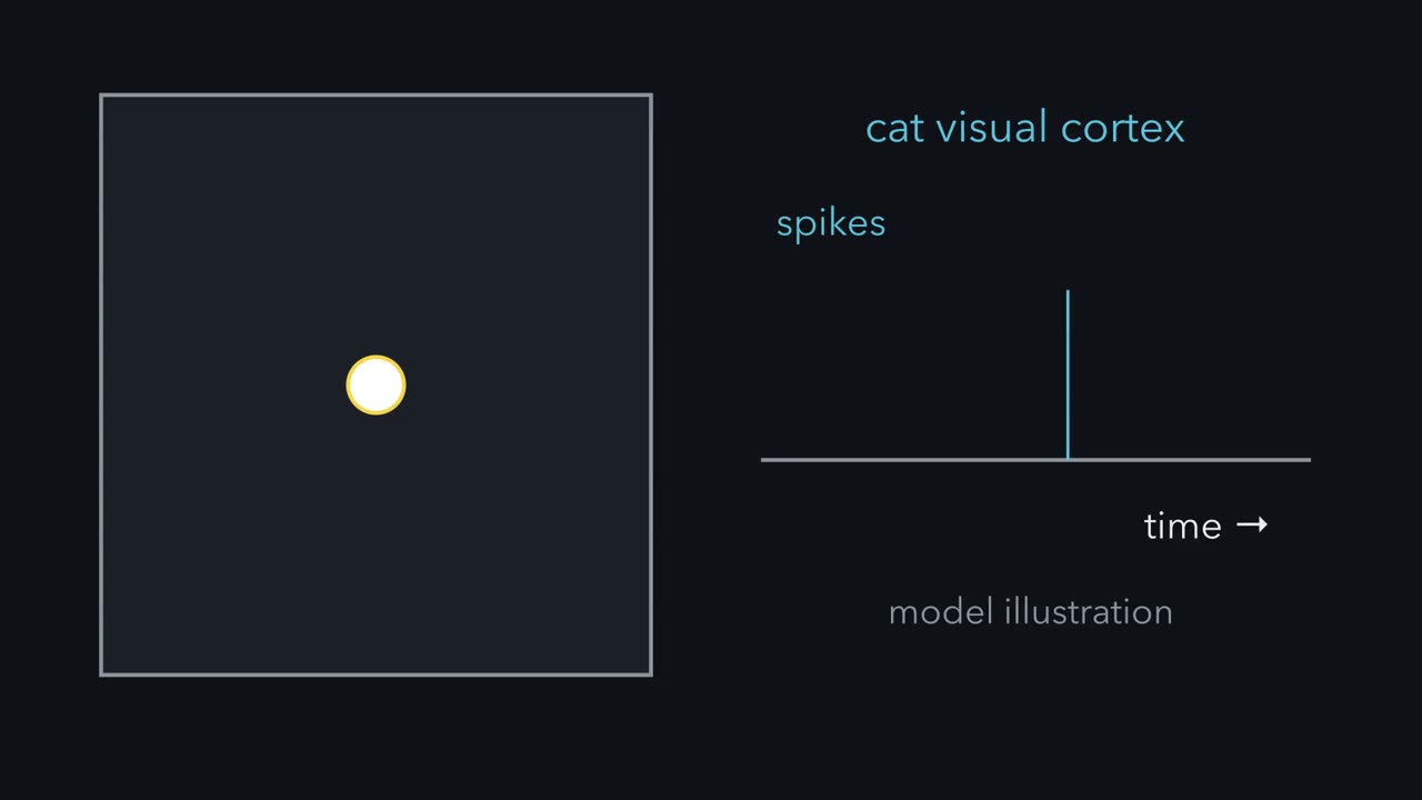 ▶ Watch Adding Up the Light · 2:17
Read the transcript of “Adding Up the Light”
Film transcript: Adding Up the Light
Spots of light drive the retina well. In cat visual cortex, the same spots often did little. A bar at the right angle drove some cells hard. Why would a bar win? Start in the retina. Every visual neuron watches one patch of the world, its receptive field. Take an ON-centre ganglion cell. Light on its small round centre excites it. Light on the ring around it, the surround, inhibits it. Shine a small spot that just fills the centre. It lands only on plus, so the cell fires faster. Now light the whole patch, centre and ring together. What will the cell do?
Very little. The centre adds plus, the ring adds minus, and the two largely cancel. Light the ring alone, and the sum goes negative, so firing drops below its spontaneous rate. When that light goes off, the cell gives a brief burst. That burst answers a change in light, which the sum alone does not capture. So here is the rule for cells like this one. Add up the light in the field. Light on an ON region counts as plus. Light on an OFF region counts as minus. A bigger sum means stronger drive. A sum near zero leaves the spontaneous rate. A positive sum can raise firing, and a negative sum lowers it, down to zero.
Where the patch sits tells you which part of the world the cell reports. How plus and minus are laid out tells you which stimulus it reports best. Cells of the thalamic relay, the lateral geniculate nucleus have fields of the same kind. It is a good first approximation for many cells in the retina and thalamus, and for simple cells in cortex. Later we find where it stops.
Keep the rule. Add up the light in the patch, plus on ON regions and minus on OFF regions.
From the film
- Add up the light in a cell's patch of the world, counting ON regions as plus and OFF regions as minus.
- A bigger sum means stronger drive, a sum near zero leaves the spontaneous rate, and a negative sum lowers firing.
- This is a good first approximation for many cells in the retina and thalamus and for simple cells in cortex.
Cut one optic nerve and one eye goes blind. Cut one optic tract, a few centimetres further back, and both eyes lose the same half of the world.
The difference comes from one crossing, and it is the first of two puzzles. The second: the retina sends the brain a mosaic of centre-surround signals that small spots drive well, yet in cat visual cortex spots often did little, while a bar of light at the right angle drove some cells hard. One rule answers both.
Two puzzles and one rule
The signals end in primary visual cortex, called V1 or striate cortex. Striate means striped: a pale band of myelinated fibres runs through it, visible to the naked eye. V1 turns the retina’s spots into oriented edges, lays them out as a map, and hands them on to dozens of further areas.
- Where. Why does a cut nerve blind one eye, while a cut tract blinds the same half of the world in both eyes?
- What. Why does a bar beat a spot in cortex?
The rule needs two terms. A neuron’s receptive field is the patch of the visual field where a stimulus changes its firing. In an ON region of the field light excites the cell, and in an OFF region light inhibits it.
The one idea to carry through this lesson. For many cells early on the path (retinal ganglion cells, lateral geniculate nucleus (LGN) cells and V1 simple cells), a good first approximation is that the cell adds up the light falling on its receptive field: plus on ON regions, minus on OFF regions.
- A bigger sum means stronger drive, and the cell turns drive into firing.
- A sum near zero leaves the spontaneous rate; a positive sum raises firing once it clears the cell’s threshold, and a negative sum lowers whatever firing there is, down to zero.
- Where the patch sits tells you which part of the world the cell reports. How the plus and minus regions are laid out tells you which stimulus it reports best.
The rule has a scope, and the lesson marks where it stops.
- It is an approximation for those cells, for steady light measured against a fixed background; some retinal and LGN cells already add light nonlinearly.
- It does not explain complex cells (below).
- It leaves out surround suppression, contrast saturation, attention, movement signals and the two cortical streams.
Phototransduction belongs to senses and cGMP, and receptive-field logic across the senses to sensory coding.
Where: every fibre reports one patch of the world
The “where” half of the rule is the tool for the pathway: each ganglion-cell fibre carries the signal from one patch of the world, so following the fibres tells you what a cut removes.
The visual field is the part of the world one eye sees while it holds still. It has a nasal half (toward the nose) and a temporal half (toward the temple). The lens inverts the image, so the temporal field falls on the nasal retina and the upper field on the lower retina. Most mistakes here come from mixing field and retina.
Ganglion-cell axons gather at the optic disc and leave the eye as the optic nerve. At the optic chiasm of humans and other primates, only the fibres from the nasal half of each retina cross to the other side. Temporal-retina fibres stay ipsilateral (on the same side). In animals with sideways-facing eyes, such as mice, most fibres cross.
| Eye | Field half | Falls on | At the chiasm | Joins |
|---|---|---|---|---|
| Left | left (temporal) field | nasal retina | crosses | right optic tract |
| Left | right (nasal) field | temporal retina | stays | left optic tract |
| Right | right (temporal) field | nasal retina | crosses | left optic tract |
| Right | left (nasal) field | temporal retina | stays | right optic tract |
Read down the last column. Behind the chiasm, each optic tract carries the contralateral (opposite) visual hemifield from both eyes: the left tract carries everything to the right of the point of gaze. The left hemisphere does not serve the right eye; it serves the right half of the world, seen by both eyes.
Predict. Which half of the world does the right optic tract carry, and from which eyes? What would cutting it do?
Check your prediction
The right tract carries the left half of the world from both eyes. The left eye’s nasal-retina fibres, which see its temporal (left) field, crossed to join it. The right eye’s temporal-retina fibres, which see its nasal (left) field, stayed on their own side and joined it too. Cutting the right tract therefore removes the left half of the field in both eyes.
The tract ends mainly in the lateral geniculate nucleus (LGN) of the thalamus, a relay that keeps the two eyes’ inputs in separate layers. LGN axons fan out as the optic radiations to V1, along the calcarine sulcus, a deep fold on the inner face of the occipital lobe. The radiations split. Fibres for the upper field sweep forward through the temporal lobe in Meyer’s loop and end below the calcarine sulcus; fibres for the lower field run through the parietal lobe and end above it. The upper field lands on the lower retina, and that lower-for-upper order holds all the way to cortex.
Four defects
Lesion logic from the nervous system map applies: along the pathway to V1, a lesion removes the signals of the fibres it cuts, so a complete cut blinds the patches of world those fibres covered. In human anatomy that gives four defects.
- Optic nerve: loss of the whole field of the eye on the same side.
- Chiasm, centre: the crossing nasal fibres of both eyes are cut, so both temporal fields are lost. This is a bitemporal hemianopia; a hemianopia is the loss of half the field.
- Optic tract, radiation or V1 on one side: the opposite half of the field in both eyes, a homonymous hemianopia (homonymous means the same side of the field in each eye).
- One branch of the radiation: a quarter field, a quadrantanopia. Meyer’s loop damage gives an upper quarter defect on the opposite side, reported after temporal-lobe surgery; parietal radiation damage gives a lower quarter.
A partial lesion gives a partial defect, and real defects are less tidy than this list: close matching between the eyes, or sparing of central vision, are tendencies only.
Design problem
Four patients each have one lesion of the visual pathway. (i) The whole field of the left eye is lost. (ii) The temporal half of the field is lost in both eyes. (iii) The right half of the field is lost in both eyes. (iv) The upper right quarter of the field is lost in both eyes. For each, locate the lesion and name the retinal halves whose output is lost.
- Field defect
- Retinal parts whose signal is lost
fibres from the nasal half of a retina fibres from the temporal half dashed grey: output lost pink V1 half: none of its input arrives (in this sketch)
Lower panel: each eye’s field as the patient sees it, the patient’s left on the viewer’s left. Hatched = lost.
In this sketch: a schematic seen from above, not an anatomical section; complete lesions only; human anatomy as the lesson gives it; each lost field part is drawn whole; the stacked boxes are a schematic of above and below the calcarine sulcus, not to scale.
Rule to keep: only nasal-retina fibres cross, so a lesion before the chiasm costs one eye its field, at the chiasm centre both temporal fields, and behind it the opposite half or quarter of the field in both eyes. Partial lesions give partial defects, close matching between the eyes and sparing of central vision are tendencies only, and this is anatomical reasoning, not clinical advice.
Saved in this browser only.
One way to do it
Draw both retinal images first (inverted both ways), then the fibres.
(i) The left optic nerve, before the chiasm: all of the left retina is cut off.
(ii) Both temporal fields: the temporal field falls on the nasal retina, and the nasal fibres of both eyes meet at the chiasm. A lesion at its centre cuts the crossing nasal fibres of both eyes.
(iii) The right half in both eyes: the right field falls on the left half of each retina, the temporal half of the left eye and the nasal half of the right eye. Those fibres join in the left optic tract, so the lesion is in the left tract, left LGN, left optic radiation or left V1.
(iv) The upper right quarter in both eyes: the upper right field falls on the lower left quarter of each retina (lower temporal in the left eye, lower nasal in the right eye). Upper-field fibres run in left Meyer’s loop to the cortex below the left calcarine sulcus, so either site fits.
This is anatomical reasoning, not clinical advice.
What: adding up the light
Now the second puzzle. Its first case is one you met in the retina. An ON-centre ganglion cell has a small round centre where light excites it and a ring around it, the surround, where light inhibits it.
Predict. Rank three stimuli for an ON-centre ganglion cell: a small spot that just fills the centre, diffuse light over the whole field, and a spot covering only the surround.
Check your prediction
The small central spot wins. It lands only on plus. Diffuse light lands on plus and minus together, and they largely cancel, so the response is weak. Light on the surround alone lands only on minus, so firing drops below the spontaneous rate. When the surround light goes off, the cell gives a brief burst; that is a response to the change in light, which a sum over steady light does not capture.
Lateral geniculate nucleus (LGN) cells have fields of the same centre-surround kind, with little preference for orientation. So the obvious next question in the late 1950s was what cortex does with them.
Why a bar beats a spot
Read the transcript of “Why a Bar Beats a Spot”
Film transcript: Why a Bar Beats a Spot
Spots of light often did little in cat visual cortex. So why would a bar at the right angle do better? David Hubel and Torsten Wiesel recorded single cells in the visual cortex of anaesthetized cats. An electrode just outside one cell counted its spikes, while light was projected onto a screen. Spots often did little. A slit or bar of light at the right angle drove some cells hard. For cells that answered small spots, they mapped the field spot by spot. In the cells they called simple cells, the field split into ON and OFF subregions. The subregions are long and narrow, side by side. A common layout is a narrow ON strip with an OFF strip on each side.
Picture the field as a grid of squares with made-up values. Plus and minus are balanced, as they roughly are in many real simple cells. Which will win: a small spot on the ON strip, or a bar lying along it? The bar wins by a wide margin. It lands on plus all along the strip. The spot collects only a little. This made-up cell fires only when the sum clears its threshold. The spot falls short. That is one reason spots often did little in cortex. Now turn the bar. It leaves the ON strip and lands on both OFF flanks, and the sum falls to near zero. Now light the whole field at once. What does the cell do?
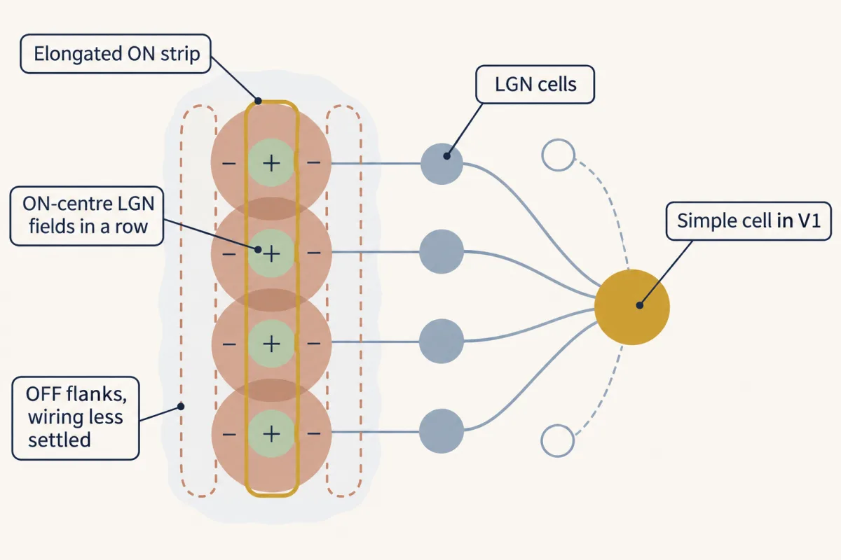
Plus and minus cancel, so diffuse light does little. A bar along one OFF strip gives a negative sum. This toy cell is already silent. A cell with spontaneous firing would slow down. So orientation selectivity is not a separate property. To a first approximation, it comes from the shape of the field. Make the strips longer but keep them just as narrow. Now the sum falls faster as the bar turns, so tuning is sharper. The threshold sharpens tuning further. Measured spike tuning is narrower than the field's sum alone predicts. How might such a field be built? Hubel and Wiesel suggested geniculate cells with ON centres in a row, all exciting one cortical cell.
That cell gets an elongated ON strip. Their surrounds could add OFF flanks, and OFF-centre cells beside the row could strengthen them. They offered this as a suggestion. Recordings in the 1990s supported the aligned input. Exactly how the flanks are built is less settled. So a bar beats a spot because it collects plus all along the ON strip. A spot collects only a little.
From the film
- A bar along a simple cell's ON strip collects plus all along it, so it beats a small spot.
- Orientation selectivity comes, to a first approximation, from the shape of the receptive field, and a threshold sharpens it further.
- Hubel and Wiesel suggested that geniculate cells with ON centres in a row feed one cortical cell, though how the flanks are built is less settled.
David Hubel and Torsten Wiesel recorded extracellularly from single cells in the visual cortex of anaesthetized, light-adapted cats: an electrode just outside one cell picked up its spikes, and they counted them while they projected spots, slits and bars of light onto a screen in front of the animal. Spots often did little; a slit or bar at the right angle drove some cells hard. Their 1962 paper in the Journal of Physiology described two main classes, and showed that for the class they called simple cells, the layout of the field predicts which stimulus drives the cell.
In simple cells that answered small, stationary spots, they mapped the field spot by spot (they also used moving slits and edges). The field is split into ON subregions, where light excites, and OFF subregions, where light inhibits and its removal excites. The subregions are long and narrow and lie side by side. A common layout is a narrow ON strip with an OFF strip on each side. Light covering an ON and an OFF region together tended to cancel.
Now apply the rule. Picture the field as a grid of squares, six squares tall: a centre column of six ON squares, each worth +1, with a column of six OFF squares on each side, each worth −0.5. The numbers are made up for teaching, but they are balanced the way many real simple cells roughly are: the OFF total equals the ON total. To turn a sum into firing, give this made-up cell no spontaneous firing and a threshold of 2: its rate is the sum minus 2 when the sum is above 2, and zero otherwise (arbitrary units).
Predict. Work out the sum for each stimulus, and decide which drives the cell: (a) a small spot covering one ON square; (b) a bar lying along the ON strip; (c) the same bar turned to lie across the field; (d) diffuse light over everything; (e) a bar lying along one OFF strip.
Check your prediction
| Stimulus | Squares covered | Sum | Rate |
|---|---|---|---|
| (a) small spot on ON | one ON | +1 | 0 |
| (b) bar along the ON strip | six ON | +6 | 4 |
| (c) bar across the field | one ON, one OFF each side | +1 − 0.5 − 0.5 = 0 | 0 |
| (d) diffuse light | six ON, twelve OFF | +6 − 6 = 0 | 0 |
| (e) bar along one OFF strip | six OFF | −3 | 0 |
The aligned bar wins by a wide margin. The small spot’s sum stays below this cell’s threshold, one reason spots often did little in cortex; real simple cells could still give weak responses to spots, enough to map their subregions. The crossing bar and diffuse light cancel. The OFF-strip bar gives a negative sum: this toy cell is already silent, but a cell with spontaneous firing would slow down. (Real OFF regions also fire a burst when their light goes off, a response to change that the steady sum does not capture.)
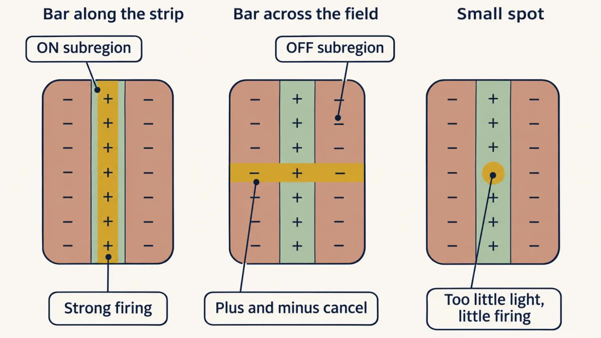
So orientation selectivity is not a separate property added on top of the field. To a first approximation, it comes from the shape of the field. Turning the bar takes it off the ON strip and onto the OFF flanks, and the sum falls. Make the subregions longer while keeping their width, and the sum falls faster as the bar turns, so the cell is more sharply tuned; what counts is length relative to width. The threshold sharpens tuning further. Only the part of the sum above it makes spikes, like the tip of an iceberg above the water, so measured spike tuning is narrower than the field’s sum alone predicts (Carandini and Ferster, 2000); applied without the threshold, the rule predicts tuning that is too broad. Circuits within cortex contribute too.
How might such a field be built?
Hubel and Wiesel suggested an answer that follows from the rule. If several lateral geniculate nucleus (LGN) cells whose ON centres lie in a row all excite one cortical cell, that cell gets an elongated ON strip. The surrounds of those LGN cells could add OFF flanks, and OFF-centre LGN cells lined up alongside could reinforce them. Their recordings measured response properties; the wiring was a proposal. Recordings in the 1990s supported the aligned-input step: ON-centre LGN cells line up with a simple cell’s ON subregions and OFF-centre cells with its OFF subregions. Exactly how the flanks are built is less settled.
Reading a tuning curve
A tuning curve plots a cell’s firing against the orientation of the bar. A narrow curve means a selective cell. Here is a made-up V1 recording. A bar at the cell’s best position is shown at six orientations, many trials each. The spontaneous rate, with no bar, is 2 spikes/s.
| Orientation (degrees) | Mean rate (spikes/s) |
|---|---|
| 0 | 2 |
| 30 | 6 |
| 60 | 24 |
| 90 | 40 |
| 120 | 22 |
| 150 | 5 |
Sketch it before you calculate: the points rise to a single peak at 90 degrees and fall away on both sides, back to the spontaneous rate at 0 degrees. Assume the response varies linearly between sampled orientations. Then you can find where the curve crosses any rate that lies between two samples:
In words Start at the first sampled angle, and add the gap between the two angles times the fraction of the way the target rate lies from the first rate to the second.
- θ“theta”
- the orientation where the line reaches the target ratedegrees
- θ1“theta one”
- the first sampled orientationdegrees
- θ2“theta two”
- the second sampled orientationdegrees
- R“R”
- the target rate you want to locatespikes/s
- R1“R one”
- the rate measured at θ1spikes/s
- R2“R two”
- the rate measured at θ2spikes/s
Sanity check If R equals R1 the fraction is 0 and θ = θ1; if R equals R2 the fraction is 1 and θ = θ2. A target rate halfway between R1 and R2 lands halfway between the two angles.
Try one number
Where does this recording’s curve cross 15 spikes/s on its rising side? Use the samples at 30 degrees (6 spikes/s) and 60 degrees (24 spikes/s).
Fraction of the way: (15 − 6)/(24 − 6) = 9/18 = 0.5.
θ = 30 + 30 × 0.5 = 45 degrees. 15 is halfway from 6 to 24, so the crossing is halfway from 30 to 60 degrees.
Need a refresher? subscripts and Greek letters · rates and “per”
Step 1: preferred orientation. 90 degrees (40 spikes/s).
Step 2: half height. Measure from the spontaneous rate: halfway from 2 up to 40 is 2 + (40 − 2)/2 = 2 + 19 = 21 spikes/s.
Step 3: where the curve crosses 21. Use the interpolation formula from the card. On the rising side, between 30 degrees (6) and 60 degrees (24): 30 + 30 × (21 − 6)/(24 − 6) = 30 + 30 × 15/18 = 30 + 25 = 55 degrees. On the falling side, between 120 degrees (22) and 150 degrees (5): 120 + 30 × (21 − 22)/(5 − 22) = 120 + 30 × 1/17 = 121.8 degrees.
Step 4: width. 121.8 − 55 = 66.8, about 67 degrees full width at half height.
Step 5: orientation index. Take 0 degrees, 90 degrees from the preferred, as orthogonal, and use the raw rates, as the index is defined.
In words The rate at the preferred orientation minus the rate at the orthogonal one, divided by their sum.
- Rpref“R sub pref”
- the firing rate at the preferred orientationspikes/s
- Rorth“R sub orth”
- the firing rate at the orthogonal orientation, 90 degrees from the preferredspikes/s
Sanity check Equal rates give 0: no preference. No firing at the orthogonal orientation gives 1. The units cancel, so the index has none.
Try one number
This recording, with raw rates: Rpref = 40 spikes/s at 90 degrees and Rorth = 2 spikes/s at 0 degrees.
Difference: 40 − 2 = 38. Sum: 40 + 2 = 42.
Index: 38/42 = 0.90, close to 1, so the cell strongly prefers its best orientation.
Need a refresher? subscripts and Greek letters · rates and “per”
For this cell the index is 0.90 (the card’s worked number shows the arithmetic). An index near 1 means the cell strongly prefers its best orientation over the orthogonal one; it does not by itself give the tuning width. With samples every 30 degrees, the width is only an interpolated estimate. Note the two baselines: Step 2 measured from the spontaneous rate, so the width describes the stimulus-driven response, while Step 5 uses raw rates. With the spontaneous rate subtracted from both rates, the index here would be 1.00, because the orthogonal response equals the spontaneous rate. Neither convention is wrong, but say which one you use; the MCAT-style question below uses raw rates.
Beyond one sum: complex cells
Read the transcript of “Anywhere in the Field, and Columns”
Film transcript: Anywhere in the Field, and Columns
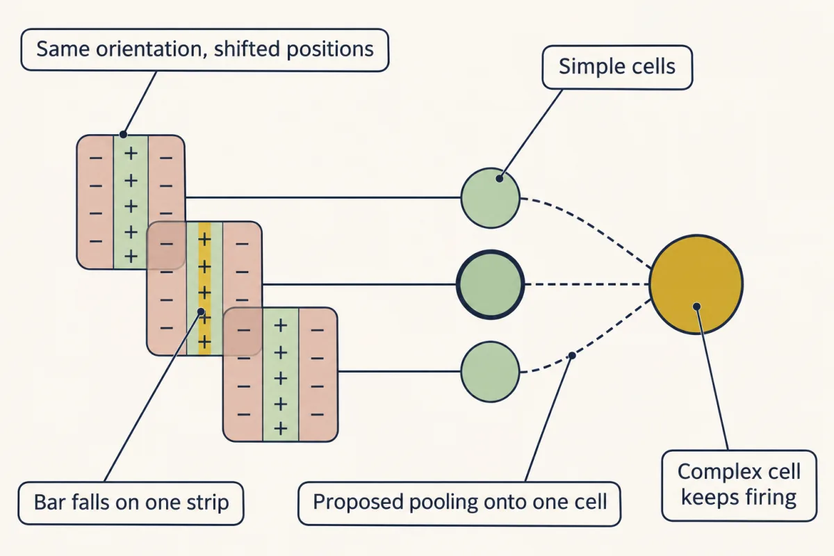
Take a simple cell's best bar and slide it sideways, off the ON strip and onto an OFF strip. What happens to the sum? It falls past zero and goes negative. This cell goes from firing hard to falling silent. Hubel and Wiesel's complex cells did. A correctly oriented bar drove them over much of the field. A bar at the wrong angle still did little. In many complex cells that answered spots, turning a spot on and turning it off excited the same places, unlike a simple cell's separate ON and OFF subregions. Other complex cells did not answer small spots. One sum cannot do that. Swap a bright bar for a dark one, and the sum flips sign. Their proposal applies the rule twice.
Several simple cells share one angle, with fields at slightly different places. All of them excite one complex cell. Where their responses overlap enough, at least one of them answers as the bar shifts. So the complex cell keeps its preferred angle and gains tolerance of position. This second step is still debated. Some complex cells receive direct geniculate input, and circuits within cortex contribute. In cat and monkey, an electrode going straight down through cortex meets cells that tend to share an angle. That is a column. Does a cell need neighbours that agree with it in order to be tuned?
No. Imaging rat visual cortex cell by cell found sharply tuned cells. Their neighbours preferred unrelated angles. This layout is called salt-and-pepper. Tuning does not need a map. So tuning does not need neighbours that agree. How each cell gets its preference is a separate question. So keep the rule and its limit. A simple cell adds up the light in its field, and the field's layout largely sets its preference. A complex cell needs more than one sum.
From the film
- A complex cell keeps its preferred angle but tolerates changes in position, which one sum cannot explain.
- Hubel and Wiesel proposed that complex cells pool simple cells of one angle at slightly different places, though this step is still debated.
- In cat and monkey, cells down a vertical track tend to share an angle, but in rat cortex sharply tuned cells sit among neighbours with unrelated preferences, so tuning does not need a map.
Hubel and Wiesel’s second class, complex cells, also preferred one orientation. Their behaviour shows where a single sum stops working.
Predict. Take the simple cell from the grid and slide its best bar sideways, off the ON strip and onto an OFF strip. What happens to the sum? Could a cell that does one sum keep firing wherever the bar lands?
Check your prediction
The sum falls from +6 to −3 as the bar crosses onto an OFF strip, so this cell goes from firing hard to falling silent. A cell with this field cannot keep firing wherever the bar lands. And no single sum can be excited by both a bright and a dark bar at the same place, because reversing the contrast flips the sign of the sum.
Complex cells did. A correctly oriented bar drove them over much of the field. A bar at the wrong angle still did little, so they do not ignore orientation; they tolerate position. In many complex cells that answered stationary spots, turning a spot on and turning it off excited the same places, unlike the separate ON and OFF subregions of a simple cell. Small spots did little for other complex cells, and in some, ON and OFF responses could be told apart but did not add and cancel the way a simple cell’s do.
Hubel and Wiesel’s proposal applies the rule twice. Several simple cells share one orientation but have fields at slightly different positions, and all of them excite one complex cell. Where their excitatory responses overlap enough, at least one of them responds strongly as the bar shifts, so the complex cell keeps orientation and gains tolerance of position, with responses weakening at gaps and at the edges of the covered span. They offered this, too, as a proposal, and how far every complex cell follows it is still debated. Some complex cells receive direct lateral geniculate nucleus (LGN) input, and intracortical circuits contribute.
The map: retinotopy, magnification and columns
V1 is retinotopic: neighbouring points in the visual field excite neighbouring points in cortex, so the field is laid out as a map. This is the “where” half of the rule written across the cortical sheet. In humans the fovea, the centre of gaze, is represented at the occipital pole, posterior to the periphery. How that map is wired up during development is covered in topographic maps.
The map is distorted. Cortical magnification is the length of cortex, in millimetres, given to one degree of visual field. It is largest at the fovea, largely because more ganglion cells serve each degree there, so more cortex is needed to map them. It falls steeply with eccentricity, the distance from the centre of gaze. In macaque, Tootell and colleagues (1988) mapped V1 with 2-deoxyglucose, a glucose analogue that marks active cells, while the animals viewed patterns of known position, and reported a maximum near the foveal representation of about 15 mm per degree. Estimates depend on the animal, the location, the direction measured and the method, so 15 is a reported macaque value, not a universal constant.
In words Distance on the cortex equals the cortical magnification times the separation in the visual field.
- distance on cortex“distance on cortex”
- how far apart the two points are represented in V1mm
- M“M”
- the cortical magnification: millimetres of cortex per degree of visual field. It falls steeply with eccentricity.mm/degree
- separation“separation”
- how far apart the two points are in the visual fielddegrees
Sanity check Units: millimetres per degree times degrees leaves millimetres. Twice the separation gives twice the cortical distance, but only while M stays the same, which is true only over a small region.
Try one number
Near the macaque fovea, with the reported 15 mm per degree, take two points 0.10 degrees apart.
15 mm/degree × 0.10 degrees = 1.5 mm of cortex.
Need a refresher? units and prefixes · rates and “per”
Worked problem: a cortical distance. Assume a locally constant magnification of 15 mm per degree near the macaque fovea. Two points 0.20 degrees apart lie 15 mm/degree × 0.20 degrees = 3.0 mm apart. Check: 3.0 mm ÷ 15 mm/degree = 0.20 degrees. Because magnification falls steeply with eccentricity, this holds only near the fovea; never apply one value across the field.
On top of the map sit columns: groups of cells, running through the thickness of the cortex, that share a property. Picture an electrode going down at right angles to the surface. In cat, Hubel and Wiesel (1962) found that cells along such a penetration tended to share an orientation preference, and that most of the cells they sampled were influenced by both eyes. In lightly anaesthetized macaque and spider monkeys (1968) they mapped orientation columns and ocular-dominance columns, groups of cells preferring one eye, along the same penetrations. They reported boundaries that seemed to be independent of each other; later work found the two maps related (see Going deeper). How eye closure in young animals reshapes ocular dominance belongs to ocular dominance and critical periods, and prenatal activity to spontaneous activity.
Predict. In the simple-cell account, a cell’s preference comes from the layout of its own inputs. Does a cell then need neighbours that share its preference in order to be tuned? Predict what imaging every cell in a patch of rat V1 might show.
Check your prediction
Ohki, Reid and colleagues (2005) imaged single cells with two-photon calcium microscopy. In rat V1, cells were orientation tuned but had no discernible local map: neighbours preferred unrelated orientations, a layout called salt-and-pepper. The same method was not blind to maps: in cat area 18, preferences were so orderly that direction-column borders were one or two cells wide. Tuning does not need a map, and columns are not universal. What generates each rat cell’s tuning is a separate question this experiment did not answer.
Beyond V1: two streams
Beyond V1, the questions change scale. In 1982 Leslie Ungerleider and Mortimer Mishkin summarized monkey evidence into two systems. Inferior temporal lesions impaired object discrimination; posterior parietal lesions impaired a landmark task that depends on spatial position. They proposed a ventral stream, occipitotemporal, for object vision, and a dorsal stream, occipitoparietal, for spatial vision: “what” and “where”. It was a working hypothesis.
Patient D.F. changed the question. She has visual form agnosia and reports the width and orientation of objects poorly. Goodale, Milner, Jakobson and Carey (1991) gave her plaques of equal area but different widths. Her width matching was poor, yet when she reached to pick the same plaques up, her grip opened in proportion to width. The object was the same; the task changed, from a report to an action (the tasks also differ in other ways; see Going deeper). Brain imaging later placed her damage mainly in lateral occipital cortex of the ventral stream on both sides, while dorsal-stream areas still responded during grasping (James and colleagues, 2003). Goodale and Milner proposed in 1992 that the ventral stream serves perception and the dorsal stream the visual control of action.
Keep its limits in view. D.F. is one patient, and one dissociation does not localize a circuit. The streams are densely interconnected, no area has a single function, and the perception-action account is widely taught but still debated. Attention returns in attention and decisions, and recording thousands of cells in large-scale neuroscience.
Carry the rule forward. Where a cell’s patch sits explains the map and the pathway defects; how its plus and minus regions are laid out explains why a bar beats a spot. Complex-cell tolerance needs a nonlinearity beyond one sum, with pooling one influential account, and areas beyond V1 need richer computations still.
Going deeper
Other targets of the optic tract
The lateral geniculate nucleus (LGN) is the main target, but other branches of the optic tract reach the superior colliculus and pretectum, and a small set of retinal axons leaves at the chiasm for the suprachiasmatic nucleus of the hypothalamus. A nucleus is a cluster of neuron cell bodies in the central nervous system.
Where the defect descriptions come from
The four defects are described for human anatomy by Patel and colleagues (2021). The upper quarter defect after temporal-lobe surgery was reported by Powell and colleagues (2005). Tract lesions often give incongruous defects, meaning the losses in the two eyes do not match closely, and V1 lesions often spare central vision, called macular sparing.
Complex cells as pooled pairs
One modern form of the pooling idea is the energy model. Two linear filters share an orientation, a spatial frequency and an envelope, but their stripes are offset by a quarter of a cycle (in quadrature). Square each filter’s signed output and add: E = u² + v². For a matched grating at phase φ (“phi”, where the stripes fall), u = A cos φ and v = A sin φ. Then E = A² cos² φ + A² sin² φ = A² (cos² φ + sin² φ) = A², because cos² φ + sin² φ = 1 for any angle. So E = A² wherever the stripes fall. Reversing the contrast flips the sign of u and v and leaves E unchanged. Adding the two outputs without squaring would give just another single sum, still sensitive to position. The energy model is not a demonstrated circuit for every complex cell, and responses to finite bars depend on the filters chosen.
Columns in cat and monkey
Cat V1 has ocular-dominance columns too: Hubel and Wiesel’s cat work noted grouping by eye preference, and Shatz, Lindström and Wiesel showed the columns anatomically in 1977.
The two column maps are related after all
Optical imaging later showed that orientation and ocular-dominance maps in monkey and cat are systematically related. Orientation pinwheel centres, the points where all orientations meet, tend to lie near the middle of ocular-dominance columns, and lines of equal orientation tend to cross ocular-dominance borders at steep angles (Bartfeld and Grinvald, 1992; Obermayer and Blasdel, 1993; Hübener and colleagues, 1997, in cat).
What a human fMRI map measures
In human fMRI maps, a population receptive field describes the pooled activity of many neurons (Benson and colleagues, 2018, 181 participants), not one cell’s field.
What the rule leaves out
Even V1 is not a pure camera. In mouse, part of its ongoing activity is related to the animal’s movements (Stringer and colleagues, 2019), and feedback from the higher area LM depends on which part of the visual field each region represents (Fişek and colleagues, 2023).
The perception-versus-action debate
D.F.’s two tasks also differ in their movements and in the feedback a grasp gives, and whether that difference explains her grasping is debated (Schenk, 2012). Critics of the perception-action account argue that the dorsal stream also supports spatial perception and memory, not only action (Kravitz and colleagues, 2011).
Your notes
Select any text in the lesson to highlight it or add a note to it. Your highlights and notes are saved in this browser and collected in your notebook.
This browser is not letting the site save anything (a private window or strict privacy settings), so highlights and notes will be lost when you leave the page.
How we measure it
Extracellular single-unit recording
A fine electrode placed near a neuron records its action potentials without entering the cell. Moving and rotating a stimulus while counting spikes maps the cell's receptive field and tuning. Each isolated unit is one neuron, though one electrode can pick up a few units at once, and the method favours large, active cells.
2-deoxyglucose metabolic mapping
A radioactive glucose analogue is taken up by active neurons and trapped. If an animal views a chosen pattern during the infusion, autoradiographs of the cortex show where activity was high, giving a map of the whole area for that stimulus. It measures metabolism summed over the session, not spikes or connections.
Two-photon calcium imaging
A calcium-sensitive indicator in cortical neurons is imaged through a cranial window with a focused near-infrared laser that excites the indicator mainly in a tiny focal volume, scanned across the tissue. Hundreds to thousands of cells can be followed at once, so the preferences of neighbouring cells can be compared directly.
Lesions and matched perception and action tasks
In monkeys, a cortical area is removed and performance on tasks that depend on object identity or spatial position is compared. In patients, the same object is used for a perceptual report and for an action, so a dissociation points to different uses of the same visual input.
Practice questions on this lesson (3) → MCAT-style, original, each with an explanation
Where this lesson fits
Before thisReview first
- The Map: How the Nervous System Is OrganizedThis course · Lesson 1
You need the lesion logic and the map of pathways from there to predict what a cut removes.
- Principles of Sensory CodingThis course · Lesson 9
Receptive fields and lateral inhibition there set up the ON and OFF centre-surround idea this lesson builds on.
- The RetinaThis course · Lesson 10
The ON-centre and OFF-centre ganglion cells there are the inputs whose signals cortex adds up here.
After thisStudy next
- Attention, Executive Control and DecisionsThis course · Lesson 25
It returns to the dorsal and ventral streams and asks what higher visual areas do with attention.
- Recording Many Neurons: Imaging, Arrays and AtlasesThis course · Lesson 27
It shows how recording thousands of cells tests tuning and column maps like those seen in cat, monkey and rat.
- Plasticity, Networks and ConsolidationThis course · Lesson 23
Its optogenetic tagging of cells links to the ventral stream's route toward object memory.
Elsewhere on the siteFilms, simulations and method films in other courses
- Lineage tracingMethod film
Following transmitted marks along axons is how tract routes are traced; this lesson uses the pathway they reveal.
- One Cell, Two EyesFilm · Developmental Neuroscience
It shows how eye-specific columns in visual cortex are rewired by closing one eye.
- A Veto From the Null SideFilm · Sensory Systems
It shows a retinal cell computing a preferred direction, the kind of feature selectivity cortex builds on.
Suggested by an AI model from the lessons themselves, then checked. How we use AI
Finish line
Test yourself
8 questions
Practice and MCAT-style, with explained answers.
Next · Lesson 12
Hearing and Balance
The same kind of cell tells you that a violin is playing an A and that your head is turning left. How does one cell type do both jobs?
Continue →