Cell Biology · Unit 1: Seeing and testing cells
New to this? Review it at high school level: The Cell Theory and Its Evidence
Microscopy and Quantitative Images
Rewritten on : new text, flashcards and film. Your notes and highlights stay, but the text around them may have moved.
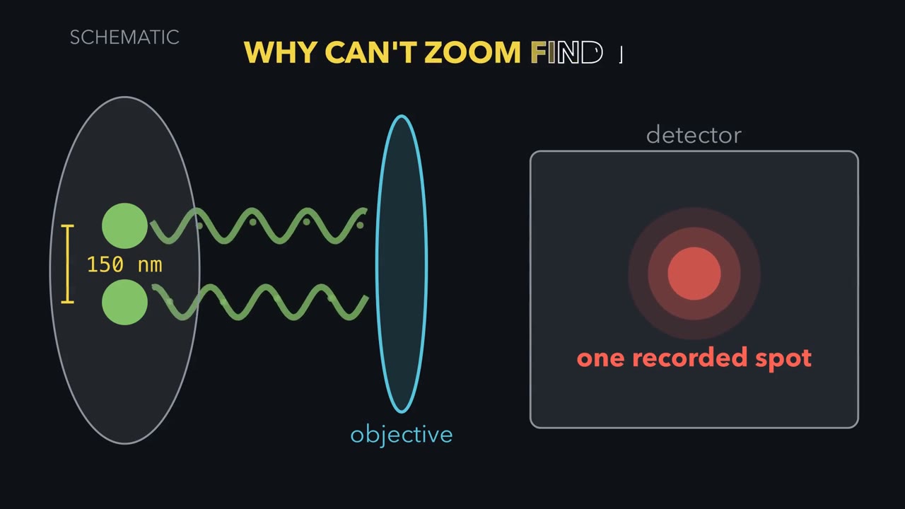
Two GFP-filled vesicles 150 nm apart look like one blob in the best ordinary light microscope. Zooming in will not split them. Why not?
Pause when the reading reaches a film, and offer to play it. Saved on this device.
Watch the film now, or keep listening
 ▶ Watch What Zoom Cannot Recover · 3:55
Read the transcript of “What Zoom Cannot Recover”
Film transcript: What Zoom Cannot Recover
These two GFP-filled vesicles are 150 nanometres apart. An ordinary light microscope records one spot. Why can software zoom not split it back into two? Follow the light from specimen to screen, and watch where the missing detail is lost.
Start with one point source. In ideal widefield fluorescence, every point becomes a blur. The screen shows a bright centre with faint rings, an Airy pattern. This computed green curve is its intensity across the screen. Why does the point spread?
Light diffracts at the objective opening. A finer pattern bends light through wider angles. The lens collects only a cone, so some information from fine detail misses the objective. Numerical aperture describes the width of the collected cone. In this ideal lateral model, the Rayleigh distance equals 0.61 times emission wavelength, divided by numerical aperture. Emission wavelength is the colour released by the fluorescent label. In the ideal lateral model, the Rayleigh distance gets smaller with shorter emission wavelength or higher numerical aperture. It is one resolution convention, not a universal border. Now restore both vesicles. Their separation is 150 nanometres.
For the settings shown here, the displayed Rayleigh distance is about 227 nanometres. Will the detector show two peaks, or one? Each source still makes its own blur. On the detector, their intensities add point by point. The two computed curves merge into one summed peak. At one hundred fifty nanometres, no dip survives between them. They are unresolved here, although other methods may separate them. Move the sources apart. A shallow dip opens before they reach the Rayleigh distance. At that distance, the central dip is about one quarter of peak height. That clear dip is the convention for calling two points resolved. For two ideal points, the Rayleigh distance marks a clear dip, not the first appearance of two peaks.
Return the vesicles to 150 nanometres. The detector again records one peak. Software zoom enlarges that record. It cannot add detail the optics and camera never captured. Optical magnification before the camera can change sampling; that is a different operation. Bigger display pixels cannot recover a missing dip. To separate or interpret closer objects, change how information enters the record. A confocal pinhole asks which out-of-focus light reaches the detector. Super-resolution asks how illumination or glowing molecules can encode closer detail. Electron microscopy replaces light with a different probe. Each change answers a measurement problem and brings new limits.
A microscope image is a measurement, not the specimen itself. Before trusting one, ask what was labelled, what the instrument could separate, and what the detector recorded. Software zoom makes the same record bigger. Software zoom cannot add detail the optics and camera never captured.
From the film
- In ideal widefield fluorescence, every point becomes a blur.
- In the ideal lateral model, the Rayleigh distance gets smaller with shorter emission wavelength or higher numerical aperture.
- For two ideal points, the Rayleigh distance marks a clear dip, not the first appearance of two peaks.
- Software zoom cannot add detail the optics and camera never captured.
The first film showed why two 150 nm sources become one recorded peak; now put numbers on that picture. The rest of the page tests camera sampling, methods that change the measurement, and what an image can support; each follows what enters the record.
Put numbers on the blur
Here λ is the label’s fluorescence emission wavelength, and numerical aperture (NA) describes the cone of light the objective collects. Resolution is the smallest separation at which two point objects can be distinguished under a stated criterion. The Rayleigh criterion calls them resolved when one Airy pattern’s centre falls on the other’s first dark ring.
Use the ideal widefield setup behind the first film’s 227 nm figure: GFP-like emission at λ = 520 nm, an oil objective with NA 1.40, and 100 nm of specimen per camera pixel. These are exercise values, not a measured point-spread function (the instrument’s response to a point); aberrations and thick samples can do worse.
Step 1, lateral resolution.
d = 0.61 × 520 / 1.40 = 317.2 / 1.40 = 226.6 nm, about 0.23 µm
The vesicles are 150 nm apart, below 226.6 nm, so they are unresolved by this criterion.
Step 2, camera sampling. Optics can preserve detail that a camera then samples too coarsely. A useful introductory rule is at least two camera pixels across one resolved distance.
Predict. Which camera samples d = 226.6 nm adequately by that rule: 100 nm specimen pixels, 150 nm specimen pixels, or both?
Check your prediction
The 100 nm camera gives 226.6 / 100 = 2.27 pixels across d, so it just meets the rule. The 150 nm camera gives only 1.51 pixels across d, so the camera loses detail that the optics could pass.
Step 3, change the objective. With the same 520 nm emission but NA 1.00, d = 317.2 nm. Losing 0.4 in NA costs about 90 nm of lateral resolution in this model.
Step 4, look along the optical axis (the depth direction). The first film used the simple lateral case; here is the fuller three-dimensional one. With immersion index n = 1.515, the approximate axial estimate is
dz ≈ 2λn/NA² = 2 × 520 × 1.515 / 1.40² = 804 nm
That is about 3.5 times the lateral value. A point’s three-dimensional blur is therefore elongated along the optical axis.
- sum of the two blurs
- each point’s own blur
- true position of each point
- camera pixels
- d (lateral) = 0.61 λ / NA
- Pixels per d
- Separation ÷ d
- Resolved? (separation ≥ d)
- Sampled? (≥ 2 pixels per d)
Keep the rule: for an ideal widefield microscope, by the Rayleigh convention two points closer than the lateral d = 0.61λ/NA count as unresolved, and a common introductory rule asks for at least two camera pixels per d; enlarging the picture afterwards adds neither. The pixel grid is centred on the midpoint of the pair. The blur curves are Airy patterns drawn in this sketch in relative units, with the first dark ring at d. These are ideal-model numbers; a real instrument or a thick sample does worse.
Change the measurement, not the zoom
Reminder: in the scoped widefield model, λ and numerical aperture (NA) set the Rayleigh distance. Once the camera samples finely enough, further magnification and software zoom only enlarge the record: magnification without resolution is empty magnification. To do better, change the measurement.
Remove out-of-focus haze
Widefield collects fluorescence throughout the illuminated depth, producing haze above and below focus in thick, densely labelled specimens. A confocal microscope scans a focused spot; a detector pinhole blocks most out-of-focus light. Each scan is an optical section, and a stack can reconstruct a three-dimensional cell, one way to measure organelle volumes. The previous lesson’s volumes came from other methods, including areas in electron-microscope sections.
Predict. If a smaller confocal pinhole rejects more out-of-focus light, why not close it as far as possible?
Check your prediction
Below one Airy unit—a pinhole as wide as the Airy pattern’s central disc—a smaller opening can buy modest resolution but costs signal. The main gain is optical sectioning and contrast; a conventional confocal remains diffraction limited, unable to separate arbitrarily close points.
Use electrons for finer structural detail
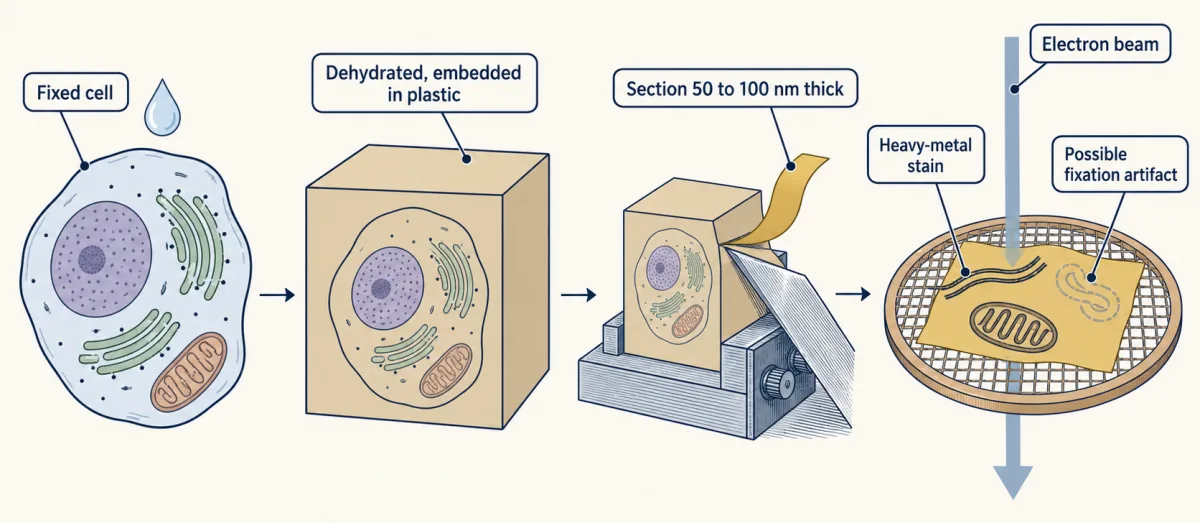
Electron microscopes focus an electron beam with magnetic lenses. Transmission EM (TEM) sends it through a thin specimen. Conventionally, cells are fixed, dehydrated, plastic-embedded, cut into 50 to 100 nm sections and stained with heavy metals. TEM can show membranes and organelles, but its image is a two-dimensional projection of dead, prepared tissue; fixation can create artifacts. Scanning EM (SEM) rasters a coated surface to show its shape.
In cryo-EM, rapid freezing traps water as glass-like vitreous ice rather than crystals. Most near-atomic cryo-EM structures come from averaging many images of purified particles. Thinned frozen cells show molecules in place, usually at lower resolution. Averaging many copies of an abundant complex such as the ribosome has produced near-atomic structures inside human cells, but not an atom-by-atom whole cell.
Encode close fluorescent emitters
Super-resolution changes what reaches the record without making diffraction disappear.
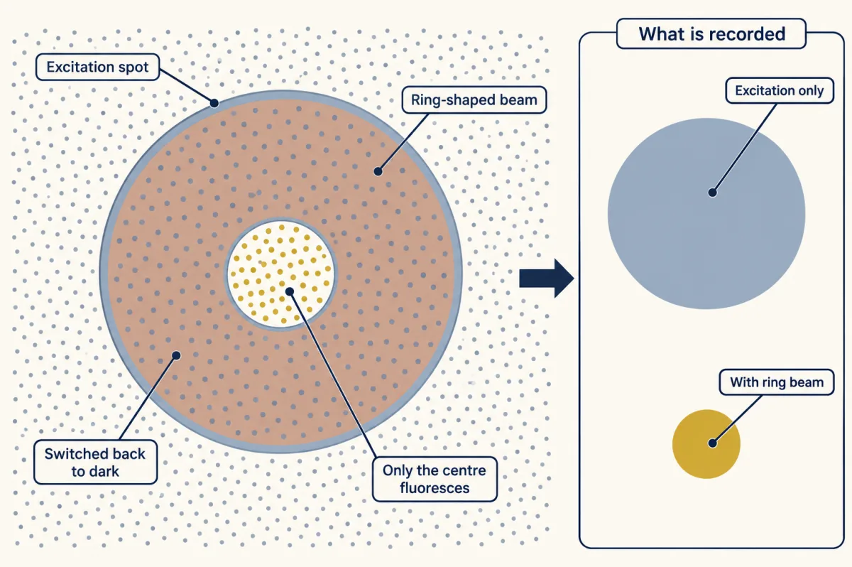
- STED uses a ring-shaped depletion beam to force excited dyes around the focus back to the dark state by stimulated emission, leaving a smaller centre able to fluoresce.
- SIM uses striped illumination to shift finer detail into the range the objective can pass, then computes an image.
- PALM and STORM switch on sparse fluorophores so nearby molecules do not glow together, estimate each isolated blur’s centre, and combine positions from thousands of cycles.
Predict. One isolated molecule makes a broad blur, but its centre is estimated to 10 nm. Does that mean two molecules 50 nm apart are resolved when they glow together?
Check your prediction
No. The 10 nm value is localization precision, the uncertainty in one isolated centre, not resolution between simultaneous emitters. PALM and STORM separate neighbours in time. Final resolution also depends on label density and size, drift and blinking; one fluorescent protein may be counted several times. With enough photons, an isolated centre can be found to a few nanometres, and shot-noise-limited uncertainty falls as 1/√N for N detected photons.
Each of these methods still ends in a record that someone must interpret.
The second film picks up here: what can two overlapping colours in that record claim?
Read the transcript of “What an Overlap Can Claim”
Film transcript: What an Overlap Can Claim
Red and green image channels overlap. Does the yellow patch mean the two proteins bind? Chapter one showed why close objects merge into one spot. Now follow the evidence from label to claim. Start with the blur from chapter one.
Across the image, it is about 230 nanometres wide. Along the depth direction, it stretches to about 800 nanometres. A yellow pixel alone cannot show that the two sources are closer than this scale. These dimensions use chapter one's green-light settings. A red channel usually has a longer emission wavelength and a larger blur. For a two-colour claim, use the measured resolution of each channel. Here is a question to hold. At typical cellular protein density, how many protein molecules would this volume contain? A handful, a few hundred, or tens of thousands?
Treat the blur as an ellipsoid. Its volume is roughly 0.02 cubic micrometres. At typical cellular protein density, it contains tens of thousands of protein molecules. So, after the controls, an in-focus overlap can support proximity within about this volume. It does not say the two proteins touch. In widefield, out-of-focus haze can create apparent overlap from farther away. Even that weaker claim needs evidence. Colour overlap is a claim about proximity. It is only as strong as each link that produced it. Check three links in turn.
First, the label. An antibody can bind the wrong protein. Signal loss after knockout supports specificity. With knockdown, the signal should fall with verified target reduction. A secondary-only sample checks nonspecific signal from the fluorescent secondary. Second, the channels. A dye's light can leak into another colour channel. That leak is called bleed-through. Single-label samples measure it, and multicolour beads test whether the channels line up. Misregistration can separate matching signals or superimpose different ones. Third, the record.
Image every condition with identical settings. Keep the relevant pixels below the detector maximum. Background subtraction removes the average background, but not its photon noise. Now return to yellow. If every link holds, an in-focus overlap supports proximity at roughly one resolution volume.
Binding is a separate claim, and it needs other experiments. Co-immunoprecipitation supports membership in the same complex, but not direct contact. A test with purified proteins addresses direct interaction. So read a colour overlap the way chapter one read the blur. Ask what was labelled, what leaked between channels, and what the detector recorded. The overlap reports what the measurement could separate, and nothing finer. Overlap supports proximity, not binding.
From the film
- A controlled, in-focus colour overlap supports proximity at roughly one resolution volume.
- In the green-light exercise, that volume is about 230 nm across and 800 nm deep, containing tens of thousands of proteins at typical cellular density.
- Overlap means something only if the label, the channels and the record each pass their controls.
- Colour overlap supports proximity, not binding; binding needs other experiments.
Read the image as a claim
The second film named the controls for each link from label to claim; here are the cases it did not work through.
1. Is the signal the claimed target?
An antibody can bind the wrong protein (see protein purification). Signal loss after target knockout supports specificity; with knockdown, the signal should fall with independently verified target reduction. A secondary-only sample checks nonspecific signal from the fluorescent secondary. A genetic tag such as GFP avoids antibodies but can alter protein location (hacking the cell and detecting a signal).
Predict. An antibody still gives the same mitochondrial pattern after its target gene is deleted, although a blot detects no target. The secondary-only sample is dark. What failed?
Check your prediction
The primary antibody is detecting something other than the target at mitochondria. The dark secondary-only control rules out the secondary antibody, but it cannot rescue the primary antibody’s specificity.
2. Are the channels separate?
Single-label samples measure bleed-through (one dye’s light leaking into another channel), and multicolour beads test whether the channels are aligned, or registered.
3. Are intensities comparable?
The second film gave the rules: identical acquisition, pixels below the detector maximum, and background subtraction that leaves photon noise. The hard case is saturation.
Predict. Treated cells contain many pixels at the detector maximum. Can their mean fluorescence be compared quantitatively with unsaturated control cells?
Check your prediction
No. A saturated pixel has stopped increasing with the light that reaches it, so its value no longer reports how much label is present. Background subtraction cannot restore clipped information.
4. What does overlap support?
After the label, channel and acquisition controls pass, an in-focus two-colour overlap can support proximity at roughly one resolution volume; widefield haze can create apparent overlap from farther away. For the first film’s green-light exercise, that volume is about 230 nm laterally by 800 nm axially. A red channel usually has a longer emission wavelength and a larger blur, so a real two-colour analysis needs the measured resolution of each channel. Treating the green-light volume as an ellipsoid gives roughly 0.02 µm³, which contains tens of thousands of protein molecules at typical cellular protein density. Colocalization supports proximity, not binding. The design problem asks what it would take to claim more.
Design problem
A paper shows an antibody to protein P staining mitochondria. Yellow overlap with a mitochondrial marker is offered as proof that P binds the marker. What would you require before accepting either claim?
Saved in this browser only.
One way to do it
First test the stain. In P knockout or knockdown cells imaged identically, mitochondrial signal should fall with P on a blot. Add a secondary-only control and independent placement: tagged P checked for function or biochemical fractionation placing P in mitochondria.
Then test proximity with single-label samples, registration beads and unsaturated raw images, so any overlap coefficient uses real intensities.
Passing those tests places the proteins only within one resolution volume (about 230 nm laterally by 800 nm axially here). Co-immunoprecipitation supports the same complex, and a proximity method supports close approach; neither proves direct contact. Purified-protein binding tests direct interaction, and interaction-breaking mutations should remove binding without changing protein amount or location.
Going deeper
The optical assumptions, sampling convention and experimental exceptions behind the main line.
Where NA and the Airy pattern come from
Light diffracts through the objective’s circular opening, so one point forms a bright disc with faint rings, an Airy pattern. Two independent emitters produce patterns whose intensities add. Ernst Abbe’s 1873 theory described fine detail sending light to wider angles; an objective can rebuild only the detail carried by light it collects.
Numerical aperture is
NA = n × sin θ
Here n is the refractive index between sample and lens, and θ is half the collected cone angle. In air n = 1.00, so NA cannot exceed 1. Immersion oil has n ≈ 1.515, allowing high-NA oil objectives near 1.4. Deep in thick, watery samples, a water objective that better matches the sample can give a sharper image. A fluorescent label absorbs one colour and emits a longer wavelength; that emission wavelength sets the detected blur.
That is why “the light limit is 200 nm” is incomplete: state the wavelength, NA, direction and criterion.
Rayleigh and Nyquist are different questions
The two-pixel rule in the main line is introductory. Strict Nyquist sampling follows the finest spatial frequency the objective passes. Here λ/(2NA) = 186 nm, so pixels should be about 93 nm or smaller. Thus 100 nm pixels give more than two pixels across the 226.6 nm Rayleigh distance but still slightly under-sample by this stricter rule; careful work often uses smaller pixels.
Evidence and history behind super-resolution
Hell and Wichmann proposed STED in 1994. In 2000 Klar, Jakobs, Dyba, Egner and Hell reported a fluorescent spot about 90 to 110 nm across, with smaller gains in live yeast and E. coli. Gustafsson reported a doubling of lateral resolution with SIM in 2000. PALM, STORM and FPALM were published in 2006 by Betzig and colleagues, Rust, Bates and Zhuang, and Hess, Girirajan and Mason, respectively. MINFLUX reported about 1 nm localization precision in 2017, but on DNA origami, not in a cell. The 2014 Nobel Prize in Chemistry went to Eric Betzig, Stefan Hell and William E. Moerner; no one person invented super-resolution.
Electron wavelength is not specimen resolution
At 100 kV an electron’s wavelength is around 0.004 nm, but preparation, contrast and beam damage make practical biological resolution far coarser. The probe’s wavelength is only one link in the measurement chain.
Labelling can move the target
Fixation is an experimental variable, and incomplete fixation can let labelling move proteins. In primary human lymphatic endothelial cells made to overexpress LYVE-1, antibodies clustered the receptor on unpermeabilised cells fixed with formaldehyde alone; adding glutaraldehyde largely prevented the clustering. The long argument over Golgi’s silver stain in nerve tissue, described in the neuron doctrine, was likewise an argument about what a stain reveals.
Your notes
Select any text in the lesson to highlight it or add a note to it. Your highlights and notes are saved in this browser and collected in your notebook.
This browser is not letting the site save anything (a private window or strict privacy settings), so highlights and notes will be lost when you leave the page.
How we measure it
Widefield and confocal fluorescence microscopy
A fluorescent label absorbs light of one colour and emits a longer wavelength, which is filtered and recorded. Widefield imaging collects light from the whole depth of the sample; a confocal pinhole rejects out-of-focus light, giving optical sections that can be stacked into a three-dimensional image. Both remain limited by diffraction.
Indirect immunofluorescence with specificity controls
Cells are fixed and permeabilized, a primary antibody binds the target, and a fluorescent secondary antibody binds the primary. The image means something only alongside controls: a knockout or knockdown that loses the signal, a secondary-only sample, and single-label samples to check bleed-through between channels.
Thin-section transmission electron microscopy
Cells are chemically fixed, dehydrated, embedded in plastic, cut into sections about 50 to 100 nm thick, and stained with heavy metals. The electron image is a two-dimensional projection of membranes and organelles in dead, prepared tissue, so artifacts of fixation must be ruled out.
Single-molecule localization microscopy (PALM, STORM)
Fluorophores are switched on a few at a time so that no two nearby ones glow together. Each one's centre is located from its blurred image, and the positions from thousands of cycles are plotted as the final picture. Precision improves with the number of photons collected.
Practice questions on this lesson (3) → MCAT-style, original, each with an explanation
Where this lesson fits
After thisStudy next
- Experiments That Distinguish MechanismsThis course · Lesson 3
It turns image-reading controls into experiments that test where a protein lives and whether it causes a defect.
- Membrane Organization and TopologyThis course · Lesson 4
It uses fluorescence and FRAP measurements, so careful image reading from here applies directly.
- Designing a Cell Biology ExperimentThis course · Lesson 26
It extends the controls and what-can-be-claimed reasoning to designing a full cell biology experiment.
Elsewhere on the siteFilms, simulations and method films in other courses
- What a Microscope Can ShowFilm · Biology
It shows that magnification makes an image bigger while resolution decides how much detail it holds.
- Zoom and resolveSimulation · Biology
You can zoom and resolve to see how the light-microscope limit stops two close points separating.
- The Size TestFilm · Life Science
It shows the size limit of what the eye can make out and why a microscope is needed.
Suggested by an AI model from the lessons themselves, then checked. How we use AI
Finish line
Test yourself
8 questions
Practice and MCAT-style, with explained answers.
Next · Lesson 3
Experiments That Distinguish Mechanisms
Where does a protein live, in what order does it travel, and does it cause the defect you see? Each question is best answered by a different experiment, and a pellet named 'mitochondria' is never only mitochondria.
Continue →← Lesson 1 · Cells Control Their Size: A Measured Eukaryotic Cell