Ecology and Evolution · Unit 2: Genomes, development and diversification
New to this? Review it at high school level: Classification Changes, Evidence for Evolution
History of Life: Transitions, Extinctions and Radiations
Rewritten on : new text, flashcards and film. Your notes and highlights stay, but the text around them may have moved.
Species have been dying out for as long as there has been life. So how did a planet of microbes end up with so many kinds of living things?
Pause when the reading reaches a film, and offer to play it. Saved on this device.
Watch the film now, or keep listening
Builds on:Reading Phylogenetic TreesMolecular EvolutionSpeciation: How Barriers to Gene Flow EvolveWhy these?
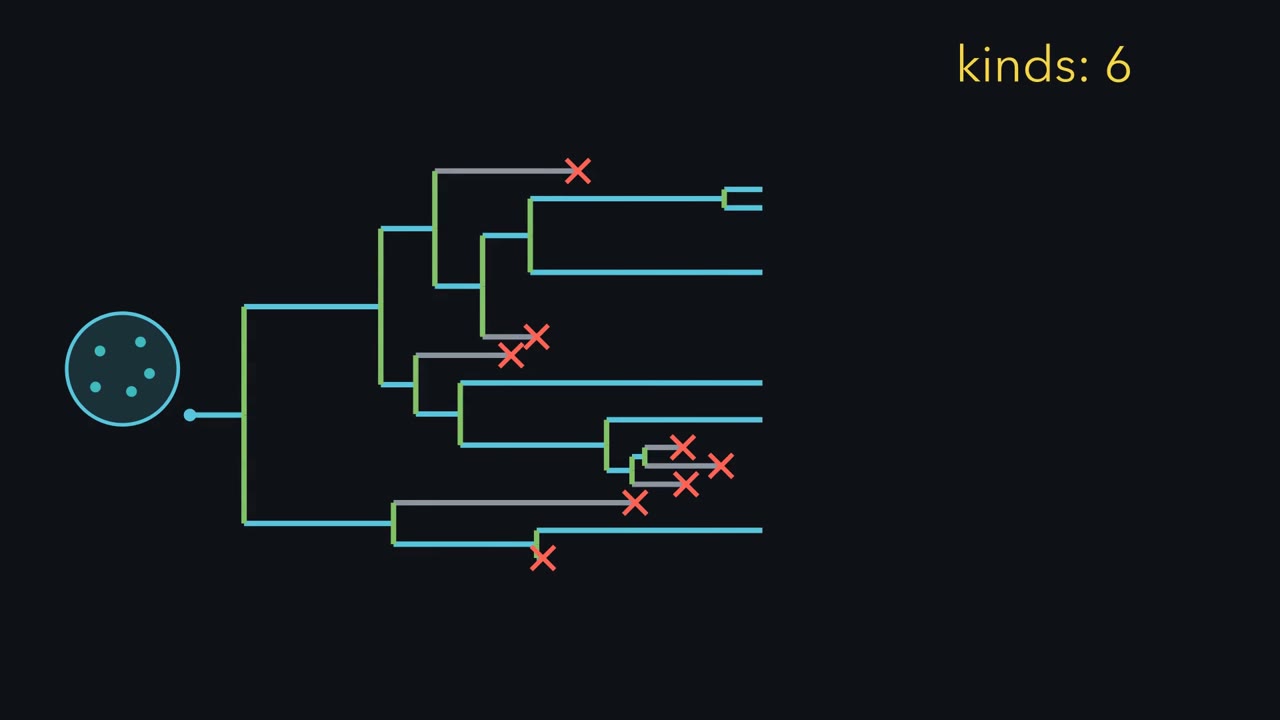 ▶ Watch Births Minus Deaths · 3:30
Read the transcript of “Births Minus Deaths”
Film transcript: Births Minus Deaths
Species have been dying out for as long as there has been life. So how did a planet of microbes end up with so many kinds of living things? In a simple model, only two events change the count of lineages. A new lineage branches off: speciation. Or a lineage ends: extinction. So the count changes by births minus deaths: the net rate r is λ minus μ. If both rates are high and nearly equal, lineages turn over fast while the total creeps up. A slow total alone cannot reveal the two rates. Now stretch the time axis back to life's earliest traces. For most of that time, life was microbial. New kinds arrive later, as flags. Each flag marks an early fossil record: by this time, at the latest.
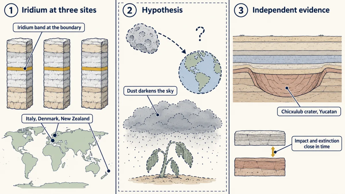
Oxygen in the air is a band instead, a change dated from both sides. In the most recent stretch, five drops are called the Big Five mass extinctions. By the benchmark on screen, each lost most species, quickly. How sharply each stands out is debated. Take the last cliff, the end of the Cretaceous. What tipped the balance? Alvarez and colleagues found extra iridium in boundary rocks at three distant sites. Iridium is scarce in Earth's crust, but richer in many meteorites. They proposed, as a hypothesis, that an asteroid struck. That predicted a crater of the right age. A buried crater, Chicxulub, was found in Mexico.
Dating tied impact and extinction closely in time. The evidence points to the impact as the trigger. Volcanic eruptions in India, the Deccan flood basalts, overlapped in time, and both causes were weighed. After the cliff, survivors can spread into emptied niches. Placental mammals diversified mainly afterward. But timing alone cannot show why. The fossil record cannot be rerun. Bacteria can. Rainey and Travisano grew one genotype of Pseudomonas fluorescens in two kinds of flask. One flask sits still, so the broth changes from the surface down. The other is shaken and stays uniform. Which will grow new types?
Only the still flask. New heritable types arose and settled into different zones. One, the wrinkly spreader, mats the surface. The shaken flask kept only the smooth type. Open niches plus heritable variation gave repeatable diversification. These were new types of one bacterium, not new species. So diversity changes by births minus deaths. Mass extinctions are short intervals when deaths far outrun births. Then survivors can diversify into the space left behind.
From the film
- The number of lineages changes by births minus deaths, speciation minus extinction (r = λ − μ); a slowly changing count alone cannot show whether the two rates are high or low.
- For most of its history life was microbial; many-celled eukaryotes, animals and land plants came later. Each fossil date means by this time, at the latest, while the oxygen date is bracketed from both sides.
- By a widely used benchmark, a mass extinction loses more than three-quarters of species in a geologically short interval; the Big Five are the standard list, though how sharply each stands out is debated.
- Iridium at distant sites, a crater of the right age and dating that ties impact to extinction point to an impact as the trigger of the end-Cretaceous extinction.
- In still broth one genotype of Pseudomonas fluorescens diversified into new heritable types; in shaken broth it did not.
The first film built one rule, births minus deaths of lineages. It left out the numbers, and they pose a puzzle.
Suppose new lineages branch off at 0.20 per lineage per million years (the speciation rate, λ, lambda) and end at 0.19 (the extinction rate, μ, mu). These are illustrative values, not measurements for any real group. A lineage then lasts about 5 million years on average (1/μ), yet the expected count grows by only 0.01 per lineage per million years. At that pace the expected count doubles in about 69 million years (ln 2 / 0.01; ln 2 is about 0.69). Turnover is fast; net change is slow. Refilling a loss of three-quarters of species means growing fourfold, about 139 million years (ln 4 / 0.01) on that average path; any one real clade is subject to chance and can follow a very different path or die out. Recovering faster needs a larger net rate: more speciation, less extinction, or both.
The one idea. In a simple birth-death model, the number of lineages changes in only two ways: speciation adds a lineage, at rate λ, and extinction removes one, at rate μ. The net rate is r = λ − μ: births minus deaths of lineages. A slowly changing count can hide two high rates that nearly cancel, or two low ones; the count alone cannot tell which. A mass extinction is a short interval when species are lost far faster than new ones arise. An adaptive radiation is the rapid diversification of one lineage into types adapted to different ecological niches (a niche is the set of conditions and resources a type uses).
Scope: this is a bookkeeping rule, not a measured history. λ and μ are averages per lineage, and for most of life’s microbial past neither rate can be recovered. The rule does not explain why oxygen built up: the Great Oxidation Event is a change in the environment, not a rate. And a drop in diversity can come from speciation stalling as well as from extinction rising.
Macroevolution is evolution above the species level: the origin, diversification and extinction of species and larger groups, built from the processes in speciation and molecular evolution. Below, Ma means millions of years ago and Ga billions of years ago.
Major transitions: new lineages, and a new atmosphere
- Microbial life, by about 3.48 Ga. Rocks in the Dresser Formation of the Pilbara, Western Australia, preserve layered mounds and microbial fabrics that Djokic and colleagues (2017) read as traces of life in hot springs on land. Reviews place a microbial biosphere on Earth by at least 3.4 billion years ago, and disputably earlier (Javaux, 2019).
- Oxygen in the air, onset about 2,460 to 2,426 Ma. The Great Oxidation Event (GOE) is the first significant buildup of oxygen in the atmosphere: when oxygen accumulated, not when oxygenic photosynthesis began, which the light reactions lesson explains. Aerobic metabolisms expanded, an ozone layer formed that would have shielded organisms in shallow surface environments from ultraviolet light, and organisms had to contend with the harmful effects of free oxygen.
- Eukaryotes (cells with a nucleus) by 1.9 to 1.4 Ga; a many-celled alga by about 1.05 Ga. The red alga Bangiomorpha pubescens, from Baffin Island, Canada, is the earliest known example of forms of multicellularity and of eukaryotic photosynthesis that still exist today (Gibson and colleagues, 2018). Its chloroplast began as an engulfed cyanobacterium (see organelles as environments).
- Animals, by about 558 Ma. Animal sterols, fat-like membrane molecules, are dominated by cholesterol and its relatives (cholesteroids). Bobrovskiy and colleagues (2018) extracted the chemical remains of such molecules from organically preserved Dickinsonia from the White Sea region, Russia. The result supported an animal affinity for Dickinsonia and its close relatives, though not for every fossil of the Ediacara biota, which spans about 571 to 541 Ma.
- Plants on land, by about 473 to 471 Ma. Rubinstein and colleagues (2010) recovered cryptospores, spores attributed to early land plants, from Middle Ordovician rocks in Argentina. Edwards and colleagues (2014) reviewed fossils that preserve such spores and found their source plants simple and millimetres high, though the affinities of cryptospores remain contentious.
What kind of date each is. The fossil entries are minimum ages: older traces could have been destroyed, never formed or not yet found. Holland (2016) stressed that preservation is uneven in space and time, so a gap in the record is not a gap in life. The GOE entry instead brackets an environmental change from both sides, using dated volcanic rocks; its exact timing is still debated (Going deeper).
Mass extinctions: when losses far outrun new species
Mass extinctions reshaped communities and biomes worldwide. A widely used benchmark (Barnosky and colleagues, 2011) sets the bar at the loss of more than three-quarters of species in a geologically short interval. That has happened five times in about the past 540 million years, the “Big Five”: the end of the Ordovician, the Devonian, the Late Permian, the Late Triassic and the end of the Cretaceous. The debate is not over whether these intervals saw heavy losses but over how sharply each stands out from background extinction, and which intervals should count (Going deeper).
End-Cretaceous, about 66 Ma. The first film traced the evidence from iridium to the Chicxulub crater, with the Deccan eruptions in India as the rival cause. Argon-argon dating by Renne and colleagues (2013) placed the impact and the extinction within 32,000 years of each other.
Predict. Does that figure mean the dying took about 32,000 years?
Check your prediction
No. The figure says the impact and the extinction happened at about the same time. It does not say how long the dying took; that needs dates within one rock section, as at Meishan below.
The weighing turned on Schulte and colleagues (2010): a single ejecta-rich layer (debris thrown out by the impact) linked to Chicxulub is spread worldwide at the boundary, it matches the onset of the extinctions in time, and the fossil patterns fit modelled darkness and cooling. They weighed both causes and concluded that the Chicxulub impact triggered the mass extinction.
End-Permian, about 252 Ma: the largest loss in the marine record. Stanley (2016) estimated that about 81% of marine species were lost in the terminal Permian crisis, a figure inferred from data on higher taxa. Burgess, Bowring and Shen (2014) dated zircons from volcanic ash beds at Meishan, China, and estimated that the extinction there lasted 60 ± 48 thousand years: tens of thousands of years, brief on a geological scale. That is one section: it constrains timing there, not the kill mechanism or worldwide synchrony, and gives a clock any proposed cause must fit.
Predict. Suppose a group of species vanished in an instant. Most individuals leave no fossil. Would each species’ last fossil lie at the extinction level, or below it?
Check your prediction
Below it. Because the record is incomplete, a species’ last fossil usually lies below where it actually vanished, so a sudden extinction is smeared backwards and looks gradual. This is the Signor-Lipps effect.
Radiations: ecological opportunity in a flask and in the record
A leading candidate cause of adaptive radiation is ecological opportunity: niches that no one is using. An extinction that removes the incumbents is one way to create it.
Two facts temper the first film’s mammals. Mammals were already diverse before the end-Cretaceous losses, and most molecular clocks (divergence dates estimated from DNA differences among living species, calibrated with fossils; more below) place many splits among placental orders in the Cretaceous. So the rise of placental mammal orders mainly after the extinction is consistent with release from competitors (survivors freed from groups that had used the same resources) but does not test it; a coincident change in climate is one alternative.
Why did the new types of Pseudomonas fluorescens last? In Rainey and Travisano’s (1998) unshaken microcosms, spatial structure supplied the ecological opportunity, and competition among the niche specialists kept them all present.
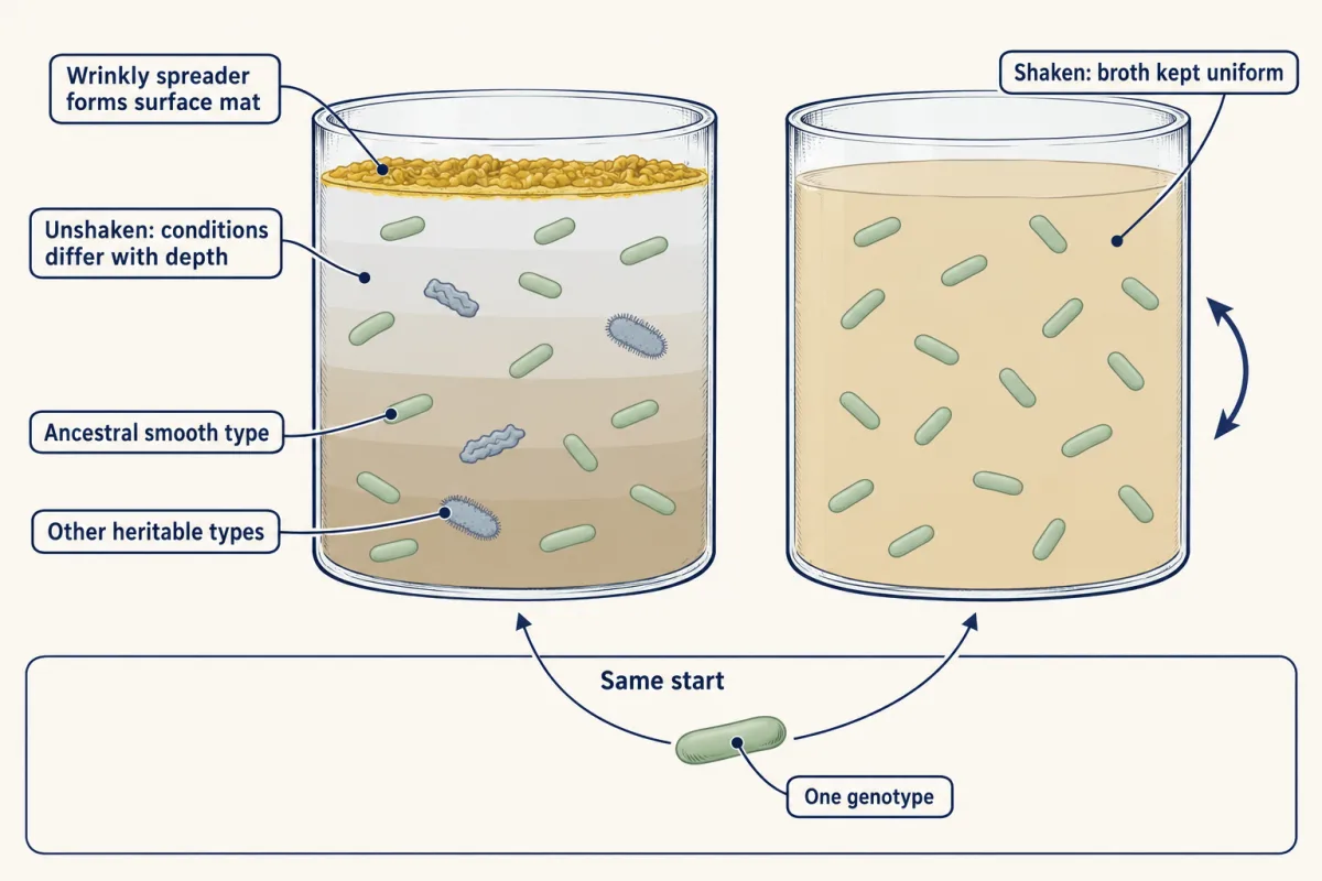
These are heritable morphs of an asexual bacterium, not new species. The flask tests the logic; it does not say every fossil radiation had the same cause.
Every claim so far has leaned on a date. The second film shows where such dates come from, and why a fossil date and an ash date are different kinds of answer.
Read the transcript of “Floors and Brackets”
Film transcript: Floors and Brackets
The first film put dates on its fossil flags and on the last cliff. But how can a rock say when a bone was buried, with no one there to see? Fossils are rarely dated directly. Often, minerals in the rocks around them are. A favourite is zircon. It crystallizes in molten rock, and an eruption carries it into volcanic ash. As zircon crystallizes, it takes up uranium but almost no lead. So nearly all the lead inside it comes from later decay. Each uranium atom has the same small chance of decaying in any given year. So half the parent atoms decay in a fixed time, the half-life. It is constant for each isotope. Watch the grid. On average, after one half-life, half the uranium has become lead.
After the next, half of what was left. The crystal keeps time from the moment it formed. Suppose the crystal stayed closed and started with no lead. Then the parent left and the lead built up count the half-lives. That count gives the age. Now take a stack of rock layers. A bed of fossils lies between two layers of volcanic ash. Each ash can be dated by its zircons. In undisturbed layers, younger ones settle on top of older ones. So the oldest lies at the bottom. How old, then, are the fossils between the two ashes?
Younger than the ash below, and older than the ash above. The answer is a bracket, not a single date. Now look at the oldest known fossil of a group. It shows the group was here by then. It does not show when the group began. Earlier members may never have been preserved, or may not have been found yet. So a first fossil is a floor, a minimum age. The group may be older. Oxygen in the air is a different kind of date. The start of the Great Oxidation Event was bracketed by dated volcanic rocks, from both sides. The clock must also fit the age.
Carbon-14 decays quickly. Long before the age of dinosaurs, too little is left to measure. So dinosaur bones are not carbon-dated. Where volcanic ash lies near them, slower clocks date those layers. Elsewhere, other methods tie the rocks to dated layers. Two kinds of date run through this lesson. Dated layers around a fossil give a bracket. A group's oldest known fossil gives a floor.
From the film
- Fossils are rarely dated directly; often minerals in nearby rocks are, such as zircon carried into volcanic ash.
- Each atom decays at random, so in each half-life about half the remaining parent atoms decay; in a closed mineral that started with no daughter, the parent left tells how many half-lives have passed.
- Dated layers below and above a fossil bed, in undisturbed rock, give a bracket, not a single date.
- The oldest fossil of a group is a minimum age: the group existed by then and may be older.
- The clock must fit the age: carbon-14 has a half-life of about 5,730 years, and after about 50,000 years too little remains to measure, so dinosaur bones are not carbon-dated.
How the dates are measured
Radiometric dating compares the parent isotope left in a mineral with the daughter isotope built up from it; the half-life is fixed for each isotope. For any date, ask four things: the measured age, the method, its uncertainty, and whether it is a point, a bracket or a minimum age.
Predict. A zircon that has stayed closed since it formed, and started with no lead, has a daughter-to-parent ratio D/P = 3. How many half-lives have passed?
Check your prediction
Two, not three: the parent left is one part in four, which is two halvings. The worked problem shows why.
Worked problem. A hypothetical zircon from an ash bed has stayed closed since it crystallized: no parent or daughter has entered or left, and, because zircon takes up almost no lead when it forms, it started with no radiogenic lead. Treat uranium-235 decaying to lead-207 as one parent and one daughter, with the rounded teaching half-life of 704 million years that the US Geological Survey uses. You measure a daughter-to-parent ratio D/P = 3.
- Recover the starting parent. Every daughter atom was once a parent atom, so P0 = P + D = P + 3P = 4P. The fraction of parent left is P/P0 = 0.25.
- Count half-lives. After n half-lives the fraction left is (1/2)n. Since 0.25 = (1/2)2, n = 2.
- Convert to years. Age = 2 x 704 million years = 1,408 million years, or 1.408 billion years.
- Check. After one half-life 50% of the parent remains; after two, 25%. Then 75% is daughter, and 75 / 25 = 3, the measured ratio.
- Date the fossils. This ash lies above a fossil bed, and a second ash below the bed is dated to 1,450 million years. In undisturbed, right-way-up layers the lower one is older, so the fossils are younger than 1,450 and older than 1,408 million years.
In this sketch: closed system, no initial daughter, one parent and one daughter. A hypothetical zircon, not a real measurement.
- Fraction of parent left, P/(P + D)
- 0.25
- Half-lives, n
- 2
- Age of upper ash
- 1,408 million years
- Fossil bed lies
- between 1,408 and 1,450 million years
Keep the rule: fraction left = (1/2)^n, age = n × half-life, and the fossils get a bracket (younger than the lower ash, older than the upper ash), not a point. This is a sketch of the logic; real geochronology uses exact decay constants and corrections.
fraction of parent left = P / (P + D) = (1/2)n, age = n x half-life
Real geochronology uses precisely measured decay constants with stated uncertainties, both uranium chains and corrections for initial lead; this exercise is a simplified model. Ash beds are not the only route: where none lie near a fossil, its rocks have to be dated by other methods.
Molecular clocks convert sequence differences among living species into divergence times, with fossils calibrating particular nodes (see reading phylogenetic trees). Parham and colleagues (2012) argued that each calibration needs an explicit justification of the fossil’s place on the tree and the age of its rock, because a misplaced or misdated fossil carries its error into the dates.
What rates the record can and cannot give
A clade, an ancestor and all its descendants, has a net diversification rate r = λ − μ, in events per lineage per million years, and a count of lineages alone cannot split it into its two parts. So biologists look at when lineages split. A time tree of living species dates each split from DNA, calibrated with fossils. Lineages that died out leave no tips, so they are missing from it.
Predict. Suppose λ and μ never changed in a clade’s history, and extinction was high. On a time tree of its living species, do new lineages appear at a steady pace, or faster toward the present?
Check your prediction
Faster toward the present. Old lineages have had a long time to die out without living descendants, so most old branches are missing; young ones have not, so almost all are still there. The count climbs steeply near today though the rates never changed: the pull of the present. Under a constant-rate birth-death model with every living species sampled, the illustrative rates from the start of the lesson (λ = 0.20, μ = 0.19) give (formula in Going deeper):
| Time before today | Rate at which lineages split on the tree of living species (per lineage per million years) |
|---|---|
| 100 million years | 0.015 |
| 20 million years | 0.045 |
| 5 million years | 0.10 |
| Today | 0.20, the full speciation rate |
With no extinction there is no pull: lineages appear at the speciation rate all the way back.
Now turn it around. A tree that climbs steeply toward the present could mean steady rates with high extinction, or speciation that rose recently with no extinction; suitably matched versions of the two fit a tree of living species exactly equally well. Unless you assume something about the rates from outside the tree (for example, that extinction was zero), the tree of survivors cannot tell them apart, and under a general model adding living species does not help (Louca and Pennell, 2020; Going deeper).
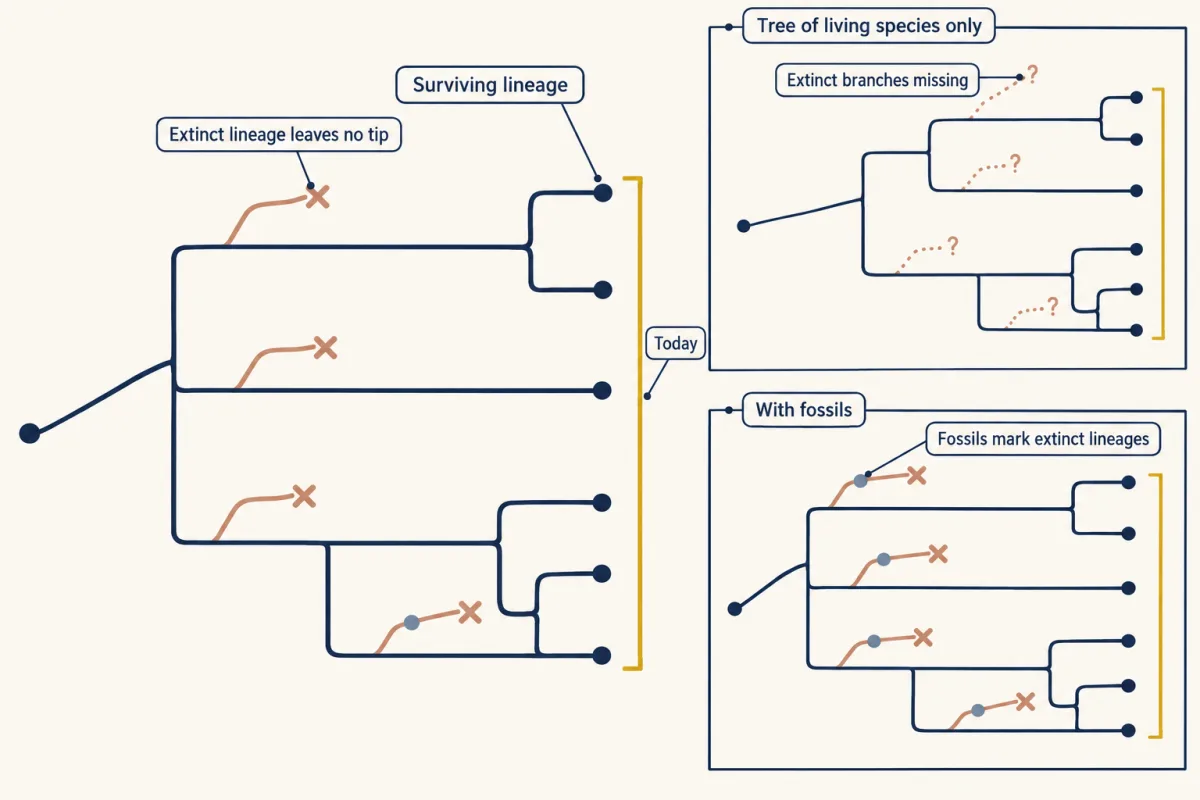
The missing information is the extinct side branches. In deep time fossils are the principal direct evidence for them, but an incomplete one, so fossil-based rate estimates must model preservation and sampling. Silvestro and colleagues (2014) built a method, PyRate, that estimates speciation and extinction from dated fossil occurrences while modelling how likely each lineage was to be preserved and found.
Design problem
Placental mammal orders diversified mainly after the end-Cretaceous extinction. A student concludes that the extinction caused the radiation by removing competitors and opening niches. What else could produce this pattern, and what data would test the student’s idea?
Saved in this browser only.
One way to do it
Alternatives. A change in climate at about the same time could have opened niches without any release from competitors. The radiation may also have begun earlier than the fossils show: recall the Cretaceous splits in most molecular clocks, and the oldest fossil of each order is only a minimum age. Unlike the flask, this event cannot be rerun with a control.
Data that would decide.
- Date the pattern. Fit dated fossil occurrences from before and after the boundary with PyRate or a similar model that estimates speciation, extinction and preservation together. Release from competitors predicts a rise in speciation that starts at the extinction horizon, not before it. A tree of living mammals alone cannot settle this.
- Check the niches. If the new mammal types took on the ecological roles of groups that died out, that supports release from competitors. If the timing of diversification tracks an independently dated climate shift instead, that supports the alternative.
- Check the clocks. Use fossil calibrations with an explicit justification of each fossil’s place on the tree and the age of its rock (Parham and colleagues, 2012), and state the uncertainty of each divergence date.
- State the fossil biases. Preservation is uneven, so a gap before the boundary is not proof of absence, and the Signor-Lipps effect makes extinctions look more gradual than they were.
Going deeper
The timeline in detail
Djokic and colleagues (2017) reported stromatolites, microbial palisade fabric and geyserite, a mineral deposit of hot springs, in the Dresser Formation rocks. Older claims need care: Allwood and colleagues (2018) reinterpreted supposed stromatolites in 3.7-billion-year-old rocks at Isua, Greenland, as more plausibly deformation structures.
The consequences of the Great Oxidation Event in the main text follow Crockford and colleagues (2026). Gumsley and colleagues (2017) bracketed the onset of the GOE using sequences of rock layers in southern Africa anchored by dated volcanic rocks. Their bracket is about 100 million years earlier than previous estimates, and they inferred that oxygen rose and fell rather than climbing once.
Gibson and colleagues (2018) used rhenium-osmium dates of sedimentary rocks above and below Bangiomorpha pubescens in the Bylot Supergroup of Baffin Island to revise its age to 1.047 billion years (plus 0.013, minus 0.017). Using that age as a calibration, their molecular clocks put the origin of the primary plastid, the chloroplast that began as an engulfed cyanobacterium, at about 1.25 Ga. That figure is a model estimate conditional on the calibration, not an observed event and not a fossil floor.
The 558 Ma age for the Dickinsonia fossils comes from earlier dating that Bobrovskiy and colleagues cite.
The early land plants that shed cryptospores belong to a pool of diversity from which bryophytes and vascular plants emerged (Edwards and colleagues, 2014).
The Big Five in the original data
David Raup and J. John Sepkoski first analysed the pattern in 1982, from a compilation of fossil marine families. They found four extinction events statistically distinct from the background rate: the end of the Ordovician, the Late Permian, the Late Triassic and the end of the Cretaceous. They also named a fifth event, in the Devonian, that stood out from the background but was not statistically significant in those data. Marshall (2023), looking back forty years later, notes that later analyses found the Big Five not statistically distinct from background rates and that there is no general agreement on which intervals count as mass extinctions; the name has stayed in standard use.
Extinction numbers
Chicxulub lies on Mexico’s Yucatán Peninsula. The iridium enrichments at the three sites behind the impact hypothesis are given in Walter Alvarez’s profile.
At Meishan, Burgess, Bowring and Shen dated zircons from five volcanic ash beds and placed the extinction between 251.941 ± 0.037 and 251.880 ± 0.031 Ma. Check their duration yourself: 251.941 − 251.880 = 0.061 million years, about 61,000 years, in line with the 60 ± 48 thousand years they estimated.
More on the flask
Kassen, Llewellyn and Rainey (2004) then varied productivity and disturbance in the same system, and diversity peaked at intermediate levels of both.
Why a tree of living species cannot settle rates
The table in the main text comes from λ·P(s), where P(s) = (λ − μ) / (λ − μ·e^(−(λ − μ)s)) is the chance that a lineage alive s million years ago has a living descendant, assuming constant rates and every living species sampled. A no-extinction model whose speciation rate rises toward today as λ·P(s) draws the same curve: the matched pair in the main text.
Louca and Pennell (2020) showed that, under a general birth-death model in which both rates may change through time, infinitely many histories are equally likely to have produced the same tree of living species, and that adding living species does not fix this even with unlimited data. The result concerns that general model: a constrained hypothesis can still be tested, but the constraint must be justified from outside the tree. PyRate lets the speciation and extinction rates vary independently through time; applied to fossil rhinoceroses, it inferred repeated shifts in both rates.
A second design problem: a tree that rises toward the present
The living species of a clade form a time tree in which the number of lineages rises steeply toward the present. A student concludes that speciation sped up recently. What else could produce this pattern, and what data would decide between the explanations?
One way to do it
Alternative. Constant speciation with high extinction gives the same shape, the pull of the present, and under a general birth-death model infinitely many histories, including ones with no speed-up, fit an extant tree equally well (Louca and Pennell, 2020).
Data that would decide.
- Add fossils. Fit dated fossil occurrences with PyRate (Silvestro and colleagues, 2014) or a similar model. Many extinct lineages and high extinction favour turnover; low extinction with recently rising speciation supports the student.
- Or justify a constraint. Without fossils, test a specific model, such as a speed-up timed to an independently dated event, and say the conclusion depends on that constraint.
- State the fossil biases. Preservation varies with rock type, environment and age, so let it vary through time in the model. First appearances are minimum ages, and the Signor-Lipps effect blurs last appearances.
Your notes
Select any text in the lesson to highlight it or add a note to it. Your highlights and notes are saved in this browser and collected in your notebook.
This browser is not letting the site save anything (a private window or strict privacy settings), so highlights and notes will be lost when you leave the page.
How we measure it
Zircon uranium-lead geochronology
Zircon crystals from volcanic ash take up uranium but almost no lead when they form, so nearly all the lead they contain accumulates by decay. Measuring parent and daughter isotopes gives the age at which the ash crystallized, and ash beds above and below a fossil horizon bracket its age.
Lipid biomarker analysis
Organic molecules are extracted from organically preserved fossils and identified by chromatography and mass spectrometry. Steroid skeletons characteristic of particular groups, such as the cholesteroids that dominate animal sterols, inform which lineage a puzzling fossil belongs to.
Experimental evolution in microcosms
Replicate populations started from one genotype are grown under controlled conditions that differ in a single factor, such as spatial structure. Comparing what evolves across treatments tests a proposed cause of diversification, and frozen samples allow evolution to be replayed.
Birth-death models fitted to fossil occurrences
Dated occurrences of fossil species are analysed with a model that includes speciation, extinction and the probability of preservation and sampling. Because extinct lineages are observed directly, such models can estimate extinction rates that a tree of living species alone cannot pin down.
Practice questions on this lesson (3) → MCAT-style, original, each with an explanation
Where this lesson fits
Before thisReview first
- Reading Phylogenetic TreesThis course · Lesson 2
You need to read a time tree and its nodes to follow what a tree of living species can show.
- Molecular EvolutionThis course · Lesson 5
Molecular clocks that date splits from DNA differences are used here to place the mammal radiation.
- Speciation: How Barriers to Gene Flow EvolveThis course · Lesson 7
Speciation is the rate λ that adds lineages in the birth-death bookkeeping used here.
After thisStudy next
- Demography and SurvivorshipThis course · Lesson 13
Survival and birth rates per age class extend the births-minus-deaths bookkeeping from lineages to individuals.
- Population Growth and RegulationThis course · Lesson 14
The exponential growth rate r and doubling time used for lineage counts are developed fully for populations.
- Global Change: Species on the MoveThis course · Lesson 24
Modern species losses and range shifts are judged against the extinction and recovery patterns seen in the fossil record.
Elsewhere on the siteFilms, simulations and method films in other courses
- How Rocks Put Fossils in OrderFilm · Biology
It shows how rock layers order fossils and how radioactive dating adds ages in years.
- Who Makes It Through the Change?Film · Life Science
It shows who survives when the environment changes, the survivors that later diversify.
- Rock layers and DNASimulation · Biology
It lets you place fossils in rock layers, the ordering that dated ash layers then bracket.
Suggested by an AI model from the lessons themselves, then checked. How we use AI
Finish line
Test yourself
8 questions
Practice and MCAT-style, with explained answers.
Next · Lesson 9
Human Evolutionary History: An African Origin and Archaic Ancestry
If our species began in Africa, why do living people whose ancestors lived outside Africa carry a little Neanderthal DNA, and how can a genome tell when it got there?
Continue →