Ecology and Evolution · Unit 3: Environments and populations
New to this? Review it at high school level: How Microbes Multiply, Populations and Carrying Capacity
Population Growth and Regulation
Rewritten on : new text, flashcards and film. Your notes and highlights stay, but the text around them may have moved.
A population of 100 growing continuously at a constant per-capita rate of 0.2 per day reaches 739 in ten days, not 300. What has to change, per individual, for that growth to stop?
Pause when the reading reaches a film, and offer to play it. Saved on this device.
Watch the film now, or keep listening
Builds on:Demography and SurvivorshipHow to Test an Evolutionary ExplanationWhy these?
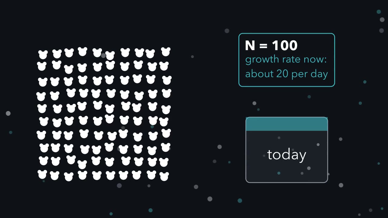 ▶ Watch Watch the Per-Capita Rate · 3:05
Read the transcript of “Watch the Per-Capita Rate”
Film transcript: Watch the Per-Capita Rate
Here is a small population, and the rate it is growing at right now. Will tomorrow's rate be the same, or faster? Look at one individual. Over day it may give birth, and it may die. Births minus deaths, per individual, is the per-capita rate. Multiply that per-capita rate by the population size, N. In a closed population, with no one moving in or out, that product is the population's growth. This one rule runs the whole film. On the left, plot the per-capita rate against N. First, hold it flat, the same value at every size.
Now watch the right panel. Each newcomer soon adds newcomers of its own. So each day's gain is bigger than the day before. By day ten, the population is far above what steady adding would give. This compounding is exponential growth, a J-shaped curve. No real population keeps this up. As numbers rise, each individual gets less food, space or shelter.
Births fall, or deaths rise. So tilt the line. Let the per-capita rate fall as N rises. The logistic model assumes it falls in a straight line. The line hits zero at a size called K, the carrying capacity. There, births balance deaths on average, so the per-capita rate is zero. Redraw the right panel with the falling line. The curve rises, steepens, then bends and levels off toward K. That is the S-shaped curve. Here is a question before we go on. On this S-curve, at what size is the population adding the most individuals per day?
Halfway to K. When the population is small, each individual adds a lot, but there are few of them. Near K, there are many, each adding little. Multiply the two at every size and plot the product in orange. It makes a hump, highest at half of K. That is where the S-curve is steepest. At K, the hump comes back down to zero.
Growth stops there because each individual's per-capita rate has fallen to zero. So the whole story sits in one teal line. Hold it flat, and growth compounds. Let it fall to zero, and growth stops at K. The straight line is the model's assumption, not a measurement. Whether real populations have a falling line must be tested in the field.
From the film
- In a closed population, growth is the per-capita rate, births minus deaths per individual, times the population size N.
- With a constant positive per-capita rate, each day's gain is larger than the last, so growth compounds.
- The logistic model assumes the per-capita rate falls in a straight line as N rises, reaching zero at the carrying capacity K.
- Total growth is largest halfway to K, where the S-shaped curve is steepest.
The first film ran one rule with the per-capita rate held flat, then falling; this text adds the units, the doubling time, life above K, and what a real brake has to be.
The one idea. A population’s growth is its per-capita rate (births minus deaths per individual, per unit time) times its size: dN/dt = (b − d) × N. A population is regulated only when that net per-capita rate falls as density (individuals per unit area) rises, from positive below some level to negative above it, so the population returns to that level from either side. This is negative density dependence, and in real populations it may act after a lag.
Scope: both models describe one closed population (no immigration or emigration) in a fixed area, so N and density rise together, with no age structure and continuous time. The exponential model holds b and d constant. The logistic holds r and K constant and assumes the net rate b − d falls in a straight line, from r at low density to zero at K, with crowding acting at once (no lag). These qualifiers hold for every model statement below.
A fixed per-capita rate: exponential growth
Write N for the number of individuals and r for the intrinsic rate of increase, the per-capita rate when resources are not limiting. With a per-capita birth rate b and death rate d, r = b − d: if b = 0.5 per year and d = 0.3 per year, r = 0.2 per year. The whole population grows at dN/dt = rN, where dN/dt (said “d N d t”) is how fast N is changing right now. Calculus turns that into a projection (the card shows what it predicts, not the derivation):
In words The population at time t is the starting population times e raised to the power r times t.
- N(t)“N of t”
- the number of individuals at time tindividuals
- N0“N zero (or N nought)”
- the number of individuals at the start, t = 0individuals
- ert“e to the r t”
- the growth factor so far: e, about 2.718, raised to the power r × t, where r is the intrinsic rate of increase (per day or per year) and t is the time elapsed in the same unit
Sanity check At t = 0, e0 = 1, so N(0) = N0. If r = 0 the population stays at N0; if r is negative it shrinks toward zero. The units of r and t must match so that r × t has no unit: an r without its time unit means nothing.
Try one number
Start with 100 individuals growing at r = 0.2 per day, and look at day 5.
r × t = 0.2 × 5 = 1, and e1 = 2.718.
N(5) = 100 × 2.718, about 272: more than one doubling (200), fewer than two (400).
Need a refresher? e and ln · powers and roots
Because r is a net rate (not a birth rate) acting at every instant, over one day the population multiplies by lambda = er: an r of 0.2 per day gives lambda = e0.2 = 1.22, a 22% rise per day, slightly more than 20% because newcomers start adding newcomers at once. Your demography lesson shows how r and lambda come from a life table.
A constant r means a constant doubling time, ln 2 / r. Doubling means ert = 2; taking the natural log of both sides (ln undoes e; see e and ln) gives rt = ln 2 = 0.693, so t = 0.693 / r. With r = 0.2 per day the population doubles every 3.47 days, whether it holds 100 individuals or 100,000.
A falling per-capita rate: the logistic model
The logistic model writes the first film’s tilted line as a brake on the per-capita rate:
In words The growth rate is r times N times one minus N over K.
- dN/dt“d N d t”
- the change in population size per unit timeindividuals per day
- r“r”
- the intrinsic rate of increase, the per-capita rate when the population is tinyper day
- N“N”
- the number of individuals nowindividuals
- K“K”
- the carrying capacity: the population size at which the model’s growth stops, in the same units as Nindividuals
Sanity check The bracket, 1 − N/K, is the brake. When N is tiny it is close to 1 and growth is nearly exponential. At N = K it is 0 and growth stops. Above K it is negative and the population falls.
Try one number
Take r = 0.2 per day and K = 1,000, as in the worked problem below, with N = 250.
N/K = 0.25, so the brake is 1 − 0.25 = 0.75.
dN/dt = 0.2 × 250 × 0.75 = 37.5 individuals per day.
Need a refresher? rates and “per”
Divide both sides by N for the per-capita rate:
(1/N) dN/dt = r(1 − N/K)
Against N this is a straight line falling from r through zero at K, the carrying capacity (real lines are often curved; Going deeper). The numbers behind the first film’s hump hold one surprise:
| N | per-capita rate r(1 − N/K), per day | total growth dN/dt, per day |
|---|---|---|
| near 0 | 0.20 (the low-density limit) | near 0 |
| 100 | 0.18 | 18 |
| 250 | 0.15 | 37.5 |
| 500 (K/2) | 0.10 | 50 (the maximum) |
| 750 | 0.05 | 37.5 |
| 900 | 0.02 | 18 |
| 1,000 (K) | 0 | 0 |
At N = 100 and N = 900 the population has the same instantaneous growth rate, dN/dt = 18 individuals per day.
Predict. Immigrants push this population to 1,200, above K. What does the model say happens next?
Check your prediction
It falls back. At 1,200 the per-capita rate is 0.2 × (1 − 1.2) = −0.04 per day, so at that moment the population is shrinking at 48 a day, and more slowly as it nears 1,000. K is a stable equilibrium, a level the population returns to from either side, not a ceiling. From below, the continuous model rises smoothly to K and never overshoots: a one-variable continuous model with instant feedback cannot.
Worked problem. Suppose a population starts at N0 = 100 individuals, with r = 0.2 per day and K = 1,000 individuals, all held constant. These numbers are illustrative, not measured for any species.
- Exponential projection at day 10. N(10) = 100 x e0.2 x 10 = 100 x e2 = 100 x 7.389 = 738.9, about 739 individuals.
- Logistic projection at day 10. The solution of the logistic equation (you can use it without deriving it) is N(t) = K / (1 + (K/N0 - 1) e−rt). Here K/N0 - 1 = 1,000/100 - 1 = 9, and rt = 0.2 x 10 = 2, so N(10) = 1,000 / (1 + 9 x e−2). With e−2 = 0.1353, N(10) = 1,000 / (1 + 9 x 0.1353) = 1,000 / 2.218 = 450.9, about 451 individuals.
- Initial logistic rate. dN/dt = 0.2 x 100 x (1 - 100/1,000) = 0.2 x 100 x 0.9 = 18 individuals per day, compared with 20 per day under the exponential model.
- Time to K/2. Set N(t) = 500: 1,000 / (1 + 9 e−0.2t) = 500, so 1 + 9 e−0.2t = 2 and e−0.2t = 1/9. Taking the natural log of both sides, t = ln 9 / 0.2 = 2.197 / 0.2 = 10.99 days.
- Peak total growth. At N = 500, dN/dt = 0.2 x 500 x 0.5 = 50 individuals per day, which is rK/4 = 0.2 x 1,000 / 4.
- Check the answers against each other. At day 10 the logistic population (451) is just short of K/2, consistent with reaching 500 at day 10.99. By day 20 the exponential model predicts 5,460 individuals (100 x e4) and the logistic about 858 (1,000 / (1 + 9 x e−4)), about one-sixth as many.
- Exponential N at the cursor
- 739
- Logistic N at the cursor
- 451
- Rate now: exponential / logistic
- 148 / 50 individuals per day
- Doubling time, ln 2 / r (exponential)
- 3.47 days
- Logistic reaches K/2 at
- 10.99 days
- Peak logistic rate, rK/4, at N = K/2
- 50 per day at N = 500
In this sketch: closed, unstructured population, constant r and K, no time lag. N0 = 100; the numbers are invented and illustrative, not measured for any species.
Rule to keep: both models start with the same per-capita rate r, but the logistic one lets it fall in a straight line to zero at K, so total growth peaks at K/2 and the population settles at K.
Now name what a field population breaks. Real populations have age structure: juveniles do not breed, so a population of mostly young animals grows more slowly than its N suggests. Feedback has time lags: food eaten this winter limits births next spring. And K changes with season, weather and food supply. These three can make a real population overshoot or cycle around K, though none always does; so can a model that steps a season at a time, if growth is strong enough (Going deeper).
Tilting the line: what counts as a brake
A limiting factor holds numbers or growth down: if adding food raises numbers compared with untouched control plots, food was limiting there. A density-dependent factor has a per-capita effect that changes with density; it tilts the line. A density-independent factor shifts the per-capita rate by the same amount at every density.
Only one direction of tilt regulates: births falling or deaths rising with density, so that net per-capita growth is positive below a level, zero at it and negative above it. The logistic meets this whenever r and K are positive, with the level at K; real feedback can arrive after a lag (the time lags above). A tilt the other way, at very low density, pushes a population away (an Allee effect, Going deeper). Neither label comes with the agent: whether a predator or a frost is density dependent is a hypothesis, tested on per-capita rates.
Predict. Add to the worked population a hazard that removes individuals at a per-capita rate of 0.05 per day at every density: a removal rate of 5 a day at N = 100, 45 a day at N = 900. Does it regulate the population?
Check your prediction
No. It kills more in total only because a fixed fraction of a bigger number is bigger. The per-capita line drops by 0.05 at every density with its slope unchanged, so it crosses zero earlier: where 0.2(1 − N/K) = 0.05, at N = 750. It lowers the level; the tilt that creates a level still comes from crowding.
So a brake shows only in per-capita rates measured across densities, which is what the second film goes looking for.
Read the transcript of “Catching the Brake”
Film transcript: Catching the Brake
The first film tilted the per-capita line by assumption. In a real forest or on a real reef, how would you catch that line tilting? Start in the Yukon, near Kluane Lake. Snowshoe hares there rise and fall in a cycle of roughly a decade.
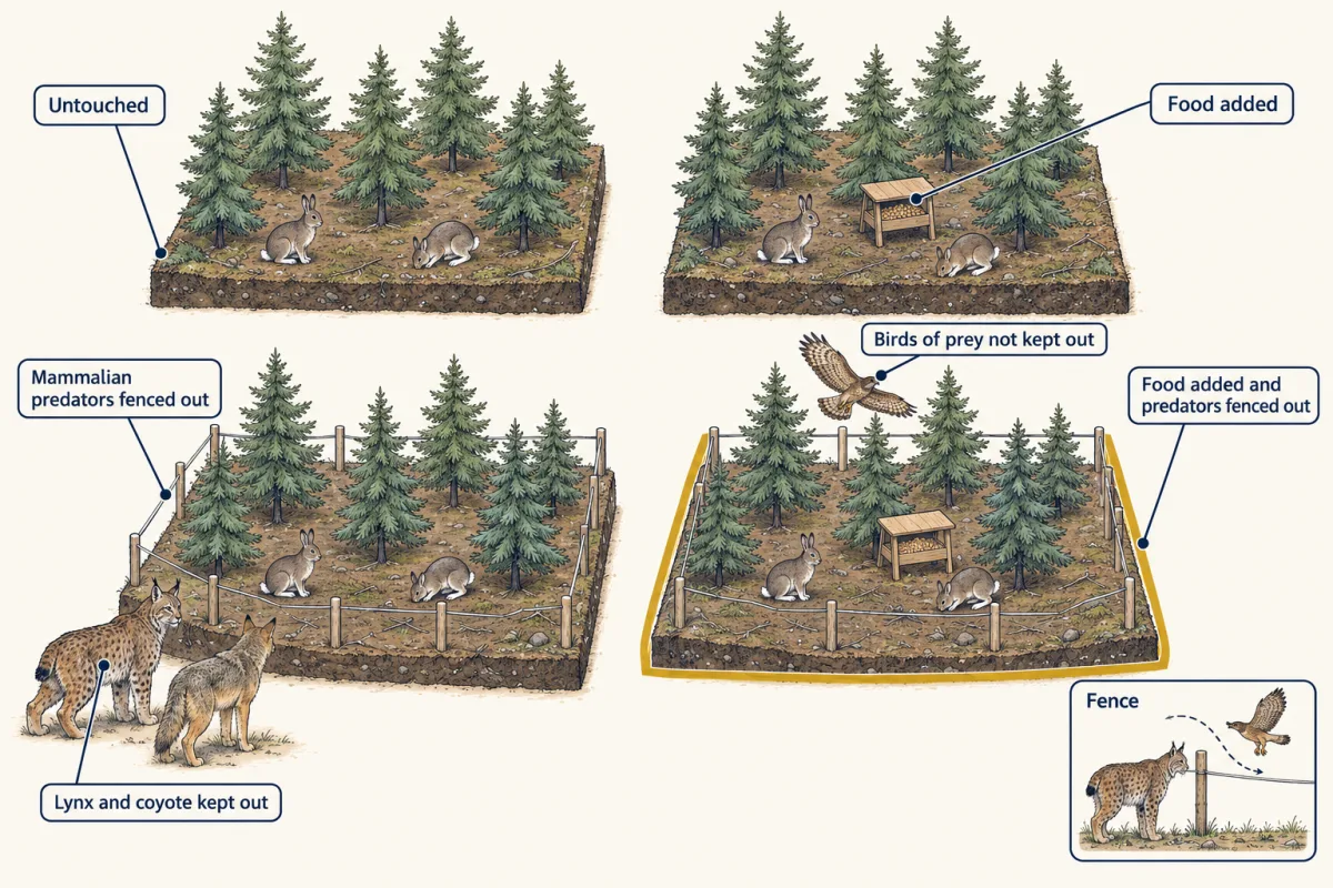
Charles Krebs and colleagues worked on blocks of forest. They added food, fenced out mammal predators, did both, or did neither. During the cycle's peak and decline, fencing out mammal predators raised hare density, and so did food. Doing both raised it far more than either alone. So food and predators both limited the hares. But were individuals doing worse at high density?
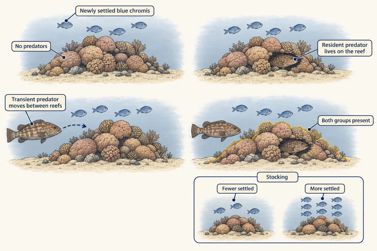
Counts of hares cannot say. For that you need a per-capita rate, measured at several densities. Mark Hixon and Mark Carr did this on small patch reefs in the Bahamas. A per-capita measure counts outcomes per individual, not heads. Here it is the fraction of young fish that died during the study on each reef. They stocked newly settled blue chromis, a small reef fish, at different densities. Some reefs got few young fish, some got many. They also crossed two kinds of predator.
Residents live on the reef. Transients swim in from open water and move between reefs. Then they plotted the fraction of young fish that died against starting density. A fraction dying is a per-capita measure, so it is teal. With both predator groups present, the line rose steeply. The more young fish that settled on a reef, the larger the share that died. That rising line is density-dependent mortality. Predators caused it on these reefs, at least when both kinds hunted there together.
Now take away one of the two predator groups, either one. Does the teal line still rise as density goes up? With only one group, no rise was detected. But one of those tests had low statistical power, too little data to catch a real slope reliably. Not detected is not the same as absent. Notice what made this a test of density dependence. Not more deaths in total, but a larger fraction of the fish dying. The hares and the chromis answer two different questions. Adding food and removing predators showed what limited the hares. The chromis showed density dependence, within one generation and across reefs. A brake is negative density dependence.
As density rises, deaths rise or births fall, so net per-capita growth falls. You find it only by measuring per-capita rates.
From the film
- Adding food and fencing out mammal predators raised snowshoe hare numbers, which shows both were limiting, but counts alone do not show density dependence.
- On Bahamian patch reefs, the fraction of young blue chromis that died rose with starting density when both resident and transient predators were present, measured across reefs within one generation.
- With only one predator group, no rise was detected, and one of those tests had low statistical power: not detected is not the same as absent.
- A brake makes net per-capita growth fall as density rises, so it is judged by per-capita measures, such as the fraction that die, not by the total number killed.
What regulates real populations
The second film skipped two limits. At Kluane each predator treatment had one fenced block, and the fences kept out lynx and coyotes but not birds of prey, so exclusion was partial.
The reef-fish slope, measured across reefs in one generation of young blue chromis, is density dependence in space. Regulation is a claim about return through time, and showing it needs evidence through time: long records, repeated density manipulations, or a tested demographic model built from measured per-capita rates.
Weather and density can also act together. Soay sheep on Hirta, in the St Kilda archipelago off Scotland, crash in some winters. Tim Coulson and colleagues reported in 2001 that lambs, adult males and adult females respond differently to density and to winter weather, so two populations of equal size under identical weather can follow different paths. The population’s makeup, which the logistic leaves out, changed the outcome.
Checking a model against data
A model earns trust by predicting populations it was not fitted to (Drake’s water fleas, Going deeper). Pearl and Reed’s 1920 logistic fitted United States census counts well, but a close fit to points you already have does not show that the mechanism in the equation is at work.
Short records are a trap. Ecologists use time series, counts of the same population year after year, and ask whether a high count is followed by a low per-capita growth rate the next year.
Predict. Take many such series and test each one alone: the pooled picture is little evidence of a fall in per-capita growth after high counts. Are most of those populations unregulated?
Check your prediction
Not necessarily. Loïc Thibaut and Sean Connolly reanalysed series from the Global Population Dynamics Database, a public collection of such records, and reported in 2020 that individual series gave little evidence of density dependence, while the series analysed together gave strong evidence. That points to low statistical power in short single series (too little data for a test to detect an effect that is there), not absent regulation.
The next two lessons, on competition and predation, build their models directly on the logistic.
Design problem
Take the Kluane result from the second film, a crossed design (each treatment alone and both together): during the peak and decline, hare densities were about 2 times control with mammalian predators excluded, 3 times with food added, and 11 times with both. Interpret the result. What does it show, what does it not show, and what would you do next?
Saved in this browser only.
One way to do it
Start with a null expectation: if food and predation acted independently and their effects multiplied, the combined treatment should give about 2 x 3 = 6 times control density. If their gains above control simply added, it would be smaller still: 1 (baseline) + 1 (predator-exclusion gain) + 2 (food gain) = 4 times. The observed 11 times exceeds both, which suggests that the two factors interact, as the authors concluded. With one fenced block per predator treatment, the interaction is suggested, not statistically tested. One reading is that extra food helps more when fewer hares are killed, and predator removal helps more when hares are well fed. Both factors limited hare density in this experiment, but that does not show that food shortage drives the cyclic decline. Krebs’s later reviews conclude that predation is the key cause, including stress from predator chases that lowers reproduction.
What it does not show: these density ratios are not r or K, and the experiment is not a test of the logistic model. The blocks were few, in one region over one run of years, so do not extend the result to all hare populations or all cycles.
Next: replicate the combined and single treatments on more blocks, ideally in another region, and measure per-capita survival and reproduction against density in each treatment. That turns “density was higher” into the per-capita evidence that regulation requires.
Going deeper
Two equilibria
With r and K positive, N = 0 is also an equilibrium of the logistic, but unstable: any population above zero grows away from it, while K is stable.
Real per-capita lines are often curved
One analysis of 1,780 animal time series (Sibly and colleagues, Science, 2005) found that per-capita growth typically fell fast at low density and then flattened, rather than falling in the logistic’s straight line. Such curves are hard to estimate from noisy counts, and sampling error in the counts can itself create spurious density dependence in a regression of growth on density.
Allee effects
At very low density the per-capita rate can instead rise as density rises, so the line slopes up before it slopes down. This is an Allee effect (positive density dependence), and the logistic leaves it out.
Chaos from the simplest model
Robert May showed in Nature in 1976 that a discrete-time logistic, with growth in seasonal steps so that this year’s crowding acts on next year’s number, can settle, oscillate, or fluctuate chaotically depending on r, with nothing random in the equation. Keep the continuous and discrete models apart: erratic counts need not mean an erratic environment.
Drake’s Daphnia test
John Drake’s 2005 analysis followed 281 laboratory populations of Daphnia magna for 104 days under food supplies of differing variability. He fitted models to some populations and tested their extinction predictions on others. Models that let demographic chance (random variation in which individuals happen to be born or die) vary with density predicted the extinctions accurately or with only slight bias; models that assumed demographic chance was the same at every density were severely biased and underpredicted them. That result belongs to those microcosms.
Your notes
Select any text in the lesson to highlight it or add a note to it. Your highlights and notes are saved in this browser and collected in your notebook.
This browser is not letting the site save anything (a private window or strict privacy settings), so highlights and notes will be lost when you leave the page.
How we measure it
Factorial field manipulation
Two or more factors, such as food and predators, are changed alone and together on replicate plots, with untouched control plots. Comparing the combined treatment with each single one shows whether the factors act independently or interact.
Predator exclusion crossed with prey density
Prey are stocked at several densities under different predator treatments, and the proportion that die is plotted against starting density. A rising slope means density-dependent mortality under that treatment; a flat slope with low power means only that none was detected.
Testing model predictions on withheld populations
A model is fitted to one set of populations and its predictions, such as which populations go extinct, are then compared with a separate set the fitting never saw. This tests what the model predicts rather than how well it can be made to fit.
Time-series analysis of abundance
Counts of one population over many years are tested for a negative relation between density and the next year's per-capita growth. Single short series often lack the power to detect that relation, so analyses that combine many series can find what single tests miss.
Practice questions on this lesson (3) → MCAT-style, original, each with an explanation
Where this lesson fits
Before thisReview first
- Demography and SurvivorshipThis course · Lesson 13
It shows how r and lambda come from births and deaths in a life table, which this lesson uses directly.
- How to Test an Evolutionary ExplanationThis course · Lesson 1
It sets out how to tell a brief change in numbers from a tested explanation, which the field-data sections here rely on.
After thisStudy next
- CompetitionThis course · Lesson 16
Its competition models are built directly on the logistic, with each species' growth braked by crowding.
- Predation and Community EffectsThis course · Lesson 17
Its predator-prey models extend logistic prey growth, and it asks why predators keep rising after prey fall.
- Movement and Spatial PopulationsThis course · Lesson 15
It relaxes the closed-population assumption here by letting movement among patches rescue populations that would otherwise go extinct.
Elsewhere on the siteFilms, simulations and method films in other courses
- Grow a population, then add limitsSimulation · Biology
It lets you grow a population and then add limits, showing growth bending toward carrying capacity.
- Run a crab cove for ten yearsSimulation · Life Science
It runs a crab population over ten years, tracking additions and losses like the per-capita rate here.
- Why Growth BendsFilm · Biology
It shows how limits slow population growth near carrying capacity, the same logistic bending.
Suggested by an AI model from the lessons themselves, then checked. How we use AI
Finish line
Test yourself
8 questions
Practice and MCAT-style, with explained answers.
Next · Lesson 15
Movement and Spatial Populations
If each pond's frogs last only about a decade, why can a region still have frogs a century later?
Continue →