Ecology and Evolution · Unit 3: Environments and populations
New to this? Review it at high school level: Populations and Carrying Capacity
Demography and Survivorship
Rewritten on : new text, flashcards and film. Your notes and highlights stay, but the text around them may have moved.
Only 10 of 100 newborn females live to age 3. Can the cohort still more than replace itself?
Pause when the reading reaches a film, and offer to play it. Saved on this device.
Watch the film now, or keep listening
Builds on:Probability, Crosses and the Chi-Square TestWhy these?
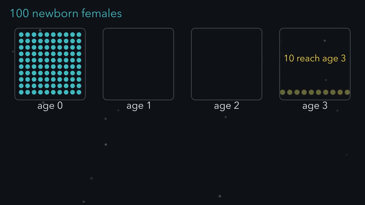 ▶ Watch Survive, Then Give Birth · 2:55
Read the transcript of “Survive, Then Give Birth”
Film transcript: Survive, Then Give Birth
Here are a hundred newborn females, all born in the same season. Only ten of them will live to age three. Can this group still more than replace itself? A group born together is called a cohort. Follow it year by year, and at each age count how many are still alive. Those that die fade to grey. Divide each count by the starting hundred. That fraction is l_x, the share of the cohort still alive at age x. Here it falls from 1 to 0.1. Survivors also give birth.
Life tables like this usually count females only, so the births we count are daughters. At each age, m_x is the average number of daughters born per living female. Here the averages are 0 in the first year, then 1, 2, and 1. Now the key step. A newborn female may not live to a given age. So her daughters there count only as far as survival allows. Multiply the share still alive by the daughters each one has. That is what an average newborn female can expect at that age. Add those pieces across her whole life. The total is R0, the daughters left by an average newborn female. Here it comes to 1.7. The dashed line marks one. At one, each female just replaces herself.
Above it, each generation is larger than the last. Below it, each is smaller. So yes, this cohort more than replaces itself. Now give the cohort a hard first winter. Only half as many females reach age one. What happens to R0?
Keep every later survival chance and birth rate the same. Every female alive at two or three first had to survive that winter. So the share alive halves at every later age, not just at age one. Every piece of R0 halves, so R0 halves too, to below the line. Survival to any age is the product of every year before it. So a loss early in life cuts every later birth. Two cautions. R0 is counted per generation, not per year. A yearly rate also needs the length of a generation. And R0 predicts long-run growth only if the rates stay fixed, and nobody arrives or leaves.
From the film
- A cohort is a group of females born together; l_x is the fraction still alive at age x, and m_x is the average number of daughters per live female at that age.
- R0, the sum of l_x times m_x over all ages, is the number of daughters an average newborn female leaves.
- If R0 is above 1 the cohort more than replaces itself; below 1 it does not. R0 is counted per generation, not per year.
- Survival to any age is the product of every earlier year's survival, so with later rates unchanged, a loss early in life lowers every later term of R0.
- R0 predicts long-run growth only if the rates stay fixed and nobody arrives or leaves.
The first film built R0 = 1.7 for a cohort, a group of females born together. Here you add the columns it skipped, turn R0 into a generation time and a yearly rate, and ask how far real counts can be trusted.
The one idea. Whether a population can replace itself depends on the net reproductive rate, R0: at each age, the chance a newborn female is alive (lx) times the average number of daughters per live female at that age (mx), added over her life. Above 1, each generation is larger than the last; below 1, smaller.
Scope: a closed female population (no migration), with rates that stay fixed, and R0 counted per generation, not per year. Wherever this page changes one rate, the others are held the same. It is a prediction from assumptions, not an observation: real vital rates change with density, weather and year.
The worked cohort, column by column
A life table summarizes how a cohort’s survival and reproduction change with age. Read the subscript x as “at age x”: nx (“n sub x”) is the number alive at exact age x, lx = nx / n0 (“ell sub x”) is the film’s survivorship, and mx its daughters per live female.
Worked problem. In this made-up data set, a closed female cohort is followed with complete records: no migration, no censoring. Each surviving female gives birth in one pulse at exact age x, before that year’s deaths, so her daughters are weighted by lx.
| x (years) | nx | lx | dx | qx | px | mx | lx mx | x lx mx |
|---|---|---|---|---|---|---|---|---|
| 0 | 100 | 1.0 | 20 | 0.20 | 0.80 | 0 | 0 | 0 |
| 1 | 80 | 0.8 | 40 | 0.50 | 0.50 | 1 | 0.8 | 0.8 |
| 2 | 40 | 0.4 | 30 | 0.75 | 0.25 | 2 | 0.8 | 1.6 |
| 3 | 10 | 0.1 | 10 | 1.00 | 0 | 1 | 0.1 | 0.3 |
| 4 | 0 | 0 | none | undefined | undefined | 0 | 0 | 0 |
The film used nx, lx and mx; each new survival column answers one question:
- dx: how many die between age x and age x + 1? dx = nx − nx+1, here 20, 40, 30, 10. They add to 100: every death is counted.
- qx: what is the chance of dying in that interval given that you reached its start? (This q is a death probability, not the allele frequency q of population genetics.)
Predict. Of the 40 females alive at age 2, 30 die before age 3. Is q2 30 out of 40, or 30 out of 100?
Check your prediction
30 out of 40, so q2 = 0.75. Only the 40 alive at age 2 were at risk. So qx = dx / nx, deaths divided by the number alive at the start of the interval (q0 = 20/100 = 0.20, q1 = 40/80 = 0.50, q3 = 10/10 = 1.00). Dividing by the original 100 gives dx/n0, not qx.
- px: what is the chance of surviving the interval? Whatever does not die survives: px = 1 − qx, here 0.80, 0.50, 0.25, 0.
Reaching age 3 means surviving year 0, then year 1, then year 2, so lx is a product of the px before it: l3 = p0 × p1 × p2 (check: l2 = 0.8 × 0.5 = 0.4). That is the product rule from probability and crosses, each stage conditional on the one before; it is why the film’s hard winter reached every later age. How births are divided among ages and offspring belongs to life histories; here mx is taken as measured. The film’s sum, in symbols:
In words R-zero is the sum, over every age, of the chance of being alive at that age times the daughters born at that age.
- R0“R zero (or R naught)”
- the net reproductive rate: daughters per newborn female, per generationdaughters per female
- sum of“sum over all ages”
- add the term for age 0, age 1, age 2 and so on
- lx“ell sub x”
- survivorship: the fraction of the cohort still alive at age x
- mx“m sub x”
- average number of daughters per live female at age xdaughters per female
Sanity check If no female lives to an age with births, every lx mx is 0 and R0 = 0. R0 = 1 means each newborn female leaves exactly one daughter, so the cohort just replaces itself.
Try one number
From the table: 0 + 0.8 + 0.8 + 0.1 = 1.7 daughters per newborn female.
Need a refresher? subscripts and Greek letters
Generation time and a yearly rate
R0 is a multiplier per generation. The cohort generation time, T, is the mean age of mothers when their daughters are born.
Predict. In the table, equal numbers of daughters (0.8 per newborn female) are born at ages 1 and 2, and a few (0.1) at age 3. Will T be exactly 1.5 years, above it or below it?
Check your prediction
Above it, at 1.59 years (card below). Ages 1 and 2 alone would average 1.5; the few daughters born at age 3 pull the mean up.
In words T is each age times the daughters born at that age, added up, then divided by all the daughters.
- T“T”
- the cohort generation timeyears
- sum of“sum over all ages”
- add the term for every age
- x“x”
- age, here in yearsyears
- lx“ell sub x”
- fraction of the cohort alive at age x
- mx“m sub x”
- daughters per live female at age xdaughters per female
- R0“R zero”
- the total daughters per newborn female, from the sum of lx mx
Sanity check It is a weighted average of ages. If every daughter were born at age 2, the top would be 2 times R0 and T would be exactly 2 years. T always lands between the youngest and oldest ages that give births.
Try one number
Top: x lx mx = 0.8, 1.6 and 0.3, which sum to 2.7. Bottom: R0 = 1.7.
T = 2.7 / 1.7 = 1.59 years.
Need a refresher? subscripts and Greek letters
Growth per year needs the intrinsic rate of increase, r, the continuous growth rate per year when rates stay fixed. A common shortcut treats T as the length of every generation: ln(1.7) is the growth rate per generation, and dividing by T gives a rate per year. Births spread over several ages make this an approximation.
In words r is roughly the natural log of R-zero, divided by the generation time.
- r“r”
- the intrinsic rate of increase, a continuous growth rateper year
- ln“natural log”
- the power you raise e (about 2.718) to in order to get the number inside
- R0“R zero”
- daughters per newborn female per generation
- T“T”
- generation timeyears
Sanity check If R0 = 1, ln(1) = 0 and r = 0: no growth. If R0 is below 1, its log is negative, so r is negative and the population shrinks. For the same R0, a shorter T gives a larger r, because the generations come round faster.
Try one number
ln(1.7) = 0.530 (check: e0.53 is about 1.7).
r = 0.530 / 1.59 = 0.334 per year.
The yearly multiplier is lambda = er = e0.334, about 1.40: roughly 40% more each year.
Need a refresher? e and ln
The shortcut is close, not exact: the exact r for this table is 0.347 per year (Going deeper), and T is not in general exactly ln(R0)/r. Population growth takes r and lambda from here.
| x | nx | lx | dx | qx | mx | lxmx | x·lxmx |
|---|
- R0 = Σ lxmx
- T = Σ x·lxmx / R0
- r ≈ ln(R0) / T
- λ = er
In this sketch: closed cohort of 100 newborn females, complete records, births in a pulse at each exact age, no female alive past age 3 (so q3 = 1.00), r approximate. Nearly equal here means q within 0.03. A sketch of the logic, not data.
Read survivorship on a log axis: a straight line means the same fraction dies each interval, not the same number; R0 is per generation, and r and λ are per year.
Whatever survival the sliders set, R0 above 1 gives a positive r and R0 below 1 a negative one; T only changes how fast. In the worked cohort, qx rose with age: 0.20, 0.50, 0.75, 1.00. What if it stayed the same at every age?
Survivorship curves and age structure
Read the transcript of “A Straight Line on a Log Axis”
Film transcript: A Straight Line on a Log Axis
In the first film, survival fed into R0. Now watch survival alone: half of this cohort dies every year. Do the same number die each year? In the first year, half of the cohort fades to grey. The grey bar below the axis counts those deaths.
The next year, half die again, but half of a smaller group. Year after year, the grey bars shrink. A constant chance of death removes the same fraction each year, not the same number. Plot the share still alive against age, on an ordinary axis. The points fall steeply at first, then the curve bends and flattens toward zero. Ecologists usually plot survival on a log axis instead. On a log axis, every halving is the same step down. So equal drops mean equal fractions lost. Watch the same points. They slide into a straight line. A constant chance of death draws a straight line on a log axis. This shape is called Type II. Two other shapes sit beside it.
Type I stays high, then plunges, because most deaths come late. Type III drops steeply, then flattens, because most deaths come early. Here is another cohort on the log axis. Its line stays almost flat, then plunges at old ages. Is the chance of dying constant, rising, or falling with age?
Rising. Few die young, and the chance of dying climbs with age, so the line bends down late. That is close to Type I. So does every animal's chance of dying rise with age? A classic reading of ageing theory said yes, for every multicellular species that breeds repeatedly. Researchers kept more than two thousand small freshwater Hydra in the laboratory, in twelve cohorts. They checked every animal daily for deaths, and for new buds.
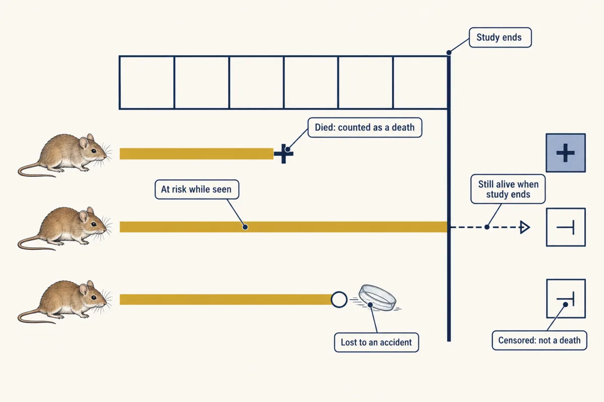
Deaths from culture accidents were not counted as natural deaths. Those animals counted as at risk while they were watched, then left the table. That is called censoring. In ten of the twelve cohorts, the yearly chance of natural death stayed near 6 in 1,000 (0.006). On the log axis that is a straight, nearly level line. Budding did not systematically fall with age. That holds for laboratory cohorts, under that counting rule. It does not show that Hydra are immortal, or that they live this way in ponds. So a straight line on a log axis means a constant chance of death. And a chance of death that rises with age is not universal.
From the film
- A survivorship curve plots l_x against age, usually on a logarithmic axis, where equal drops mean equal fractions lost.
- Type II means a constant probability of death each interval: the same fraction dies, so the number dying shrinks and the log curve is a straight line.
- Type I curves stay high and then plunge, with deaths late in life; Type III curves drop steeply early, then flatten.
- In laboratory Hydra, ten of twelve cohorts kept a yearly chance of natural death near 0.006, with no systematic fall in fertility (budding) with age.
- That is a laboratory counterexample to a universal rise in mortality with age, not evidence that Hydra are immortal.
Real species mix the film’s three ideal shapes, often with Type III juvenile losses followed by Type I adult survival, and the worked cohort, with qx rising, sits nearer Type I.
In symbols, a constant q gives lx = (1 − q)x, and taking logs turns repeated multiplication into repeated addition: log lx = x × log(1 − q), a straight line falling by the same step each year (see log scales).
A single average can hide where deaths fall, too. Life expectancy at birth is the mean length of life over all newborns, so heavy infant mortality drags it far down. In an invented population where 30% of newborns die within days of birth and the rest all live to exactly 50, life expectancy at birth is about 35 years (0.3 × about 0 years + 0.7 × 50 years), yet no adult dies at 35.
An age-structure diagram (an age pyramid) is not a survivorship curve: it shows the proportion of a population in each age class now, which depends on past births as well as survival. A pyramid with a broad base is not a Type III curve; it may be a growing population with good juvenile survival. Under the usual conditions (fixed rates, no migration, and births spread over ages so the age classes mix rather than cycle), a population converges toward a stable age distribution: the shares in each age class stop changing while the total grows or shrinks. Those shares depend on both survival and the growth rate. In a growing population each year’s newborns outnumber the last year’s, so the young are a larger share than survival alone would give.
Predict. A human population has many young people, and its fertility falls today to replacement, the level at which each generation exactly replaces itself in the long run. Does it stop growing today?
Check your prediction
No. It can keep growing for decades, because the number of women of reproductive age is still rising as the large young cohorts grow up. This is demographic momentum. The often quoted replacement figure of about 2.1 children per woman applies only where few children die before adulthood.
Where the numbers come from, and what they miss
Of 100 adult birds banded at a colony, 60 are seen there the next year. Did 40 die? Not necessarily: some may be alive and missed, some alive elsewhere. R0 is only as good as the lx and mx behind it, and there are three ways to get them.
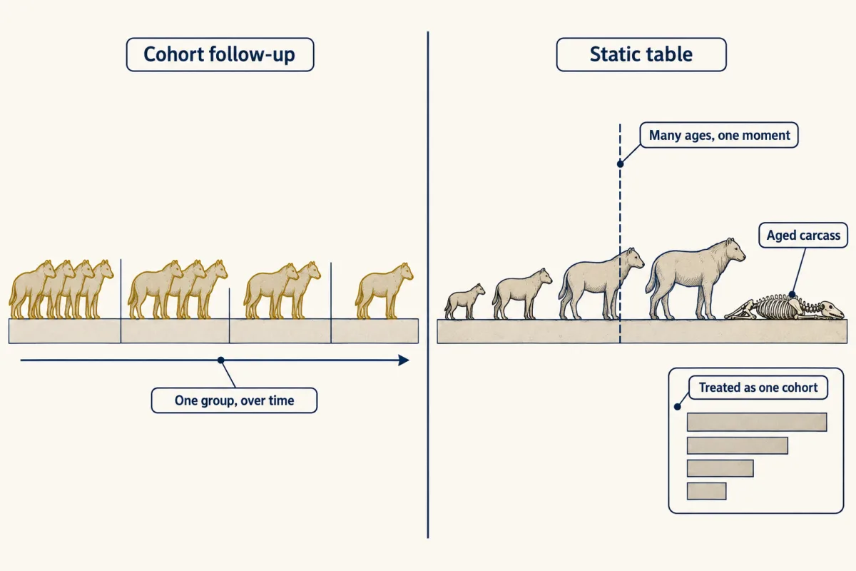
Cohort follow-up, the method the worked table assumed, marks every individual born in one period and checks, at each age, who is alive and how many daughters each has. It gives lx and mx directly, but slowly: for a long-lived species, the last member of one cohort can outlive a research career.
A static table is the shortcut: one snapshot. Age the living animals and read the number at each age as a cohort’s survivors, or age the carcasses and read the ages at death as a cohort’s deaths. Either way, animals born in different years stand in for one cohort. The simplest case where that is fair is a stationary population: about the same number born each year, and the same death rates at each age, for many years (a population growing at a known rate can be corrected; see Going deeper). Every age must also be sampled fairly, in proportion to its numbers. Young remains are fragile and easily missed, so a carcass table can undercount early deaths, and ages read from remains carry error too.
Mark-recapture, for animals you cannot watch continuously, records on repeated visits which marked animals are seen again. An animal seen after a gap was alive and missed, so across many animals the sightings and gaps let a model estimate detection separately from survival. After an animal’s last sighting, though, it usually cannot tell whether that animal died, left for good or was missed.
Each method has weak points. Some bias the estimates; others make them less certain or hide variation:
- Censoring. An animal still alive when the study ends, or lost to an accident in a study of natural deaths, is right-censored (figure below): at risk while seen, never a death. That is fair only if being censored is unrelated to the risk of dying; animals lost because they were sick or weak bias survival upward. The 2016 primate tables removed half the censored animals from the number at risk in their interval.
- Few old individuals. Small samples at old ages hide gradual changes in mortality, so the oldest ages are usually among the least certain.
- Pooled years. Tables pooled across years, like the primate tables, give average rates and hide good and bad years.
- Missing is not dead. Even with detection modelled, a survivor that left looks like a death: apparent survival is true survival multiplied by site fidelity, the chance a surviving animal stays in the study area, so permanent emigration pulls it below true survival (spatial populations takes this further).
Design problem
Return to the colony that opened this section: 60 of 100 banded adults were seen there the next year. A student concludes that adult mortality is 40% a year. Evaluate the conclusion and design a better study of adult survival.
Saved in this browser only.
One way to do it
The 0.60 is an apparent return rate, lowered by three things besides death: birds alive at the colony but not seen, birds alive that moved elsewhere for good, and birds that lost their bands.
- Detection. Search the colony on several occasions each season and for several years, and fit a Cormack-Jolly-Seber model, the standard model for such encounter histories, to each bird’s record, so that detection probability and apparent survival are estimated separately.
- Emigration. Search neighbouring colonies, or fit a subset of birds with tracking devices, to estimate permanent emigration, the fidelity term in apparent survival. In Bonelli’s eagles in Catalonia, modelling dispersal jointly shifted survival estimates for non-breeding females more than for males, by a few hundredths with wide uncertainty; breeder survival did not change (Badia-Boher and colleagues, 2023).
- Band loss. Double-mark some birds with two bands, or a band and a second mark, to estimate how often bands are lost.
- Unknown fates. Record birds never seen again as unknown fates, keeping their later missed searches in their encounter histories, not as dead.
If detection is 0.9 and fidelity 0.8, an apparent return of 0.60 would point to true survival near 0.6/(0.9 x 0.8), about 0.83, and annual mortality nearer 17% than 40%. Both values are invented to show the logic; only the study can supply the real ones.
Going deeper
The exact yearly rate
With fixed rates, the exact r solves the Euler-Lotka equation; with births in a pulse at each exact age, as in the worked table, it reads sum of λ−x lx mx = 1, where λ = er is the yearly multiplier. For the worked table λ = 1.415 and r = 0.347 per year, against 1.40 and 0.334 from the shortcut, so the shortcut r is about 4% low here (and the yearly multiplier about 1% low). Scaling every mx up or down moves λ across 1 exactly where R0 crosses 1, so the sign rule in the one idea holds exactly; only the size of r is approximate.
Census conventions
Other treatments census just before or just after the yearly breeding pulse, which changes where survival enters the formulas. Matrix models (Leslie matrices) make that choice explicit, and the exact λ is the dominant eigenvalue of such a matrix built with a consistent convention.
Static tables when a population grows
Stationarity is the simplest requirement. Strictly, a population at a stable age distribution, growing at a known rate r, can also be corrected for that growth: its older age classes were born when the population was smaller.
Your notes
Select any text in the lesson to highlight it or add a note to it. Your highlights and notes are saved in this browser and collected in your notebook.
This browser is not letting the site save anything (a private window or strict privacy settings), so highlights and notes will be lost when you leave the page.
How we measure it
Cohort follow-up (individual census)
Mark or identify every individual born in a period and record, at fixed intervals, who is alive and how many offspring each has produced. It gives l_x and m_x directly, but only for the years and conditions the cohort lived through.
Censored life-table estimation (actuarial and Kaplan-Meier)
When some individuals are still alive or lost when the study ends, their records are censored: they count as at risk for the time they were seen and are not counted as deaths. This gives fair estimates only if being censored is unrelated to an animal's risk of dying. Actuarial tables adjust the number at risk in each interval, and Kaplan-Meier curves with log-rank tests compare survival between groups.
Capture-mark-recapture (Cormack-Jolly-Seber models)
Mark animals and resight or recapture them on repeated occasions. Patterns of sightings and gaps across many encounter histories let the model estimate detection probability and apparent survival separately; permanent emigration still has to be estimated with extra information, such as encounters outside the study area.
Practice questions on this lesson (3) → MCAT-style, original, each with an explanation
Where this lesson fits
Before thisReview first
- Probability, Crosses and the Chi-Square TestGenetics and Molecular Biology · College: the core
Survival to an age is a product of each year's survival, the same product rule you use for crosses.
After thisStudy next
- Population Growth and RegulationThis course · Lesson 14
It takes the r and yearly multiplier from a life table and uses them to model exponential and logistic growth.
- Movement and Spatial PopulationsThis course · Lesson 15
It takes further how emigration and missed animals make apparent survival fall below true survival.
Suggested by an AI model from the lessons themselves, then checked. How we use AI
Finish line
Test yourself
8 questions
Practice and MCAT-style, with explained answers.
Next · Lesson 14
Population Growth and Regulation
A population of 100 growing continuously at a constant per-capita rate of 0.2 per day reaches 739 in ten days, not 300. What has to change, per individual, for that growth to stop?
Continue →