Ecology and Evolution · Unit 6: Global change and decisions
New to this? Review it at high school level: Matter Cycles, The Chesapeake Under Pressure
Global Change: Species on the Move
Rewritten on : new text, flashcards and film. Your notes and highlights stay, but the text around them may have moved.
A mountain warms 0.3 C in a decade. How far uphill must a beetle's range shift to stay as cool as before?
Pause when the reading reaches a film, and offer to play it. Saved on this device.
Watch the film now, or keep listening
Builds on:Climate, Biomes and Environmental VariationDistributions, Niches and TolerancesNutrient CyclingWhy these?
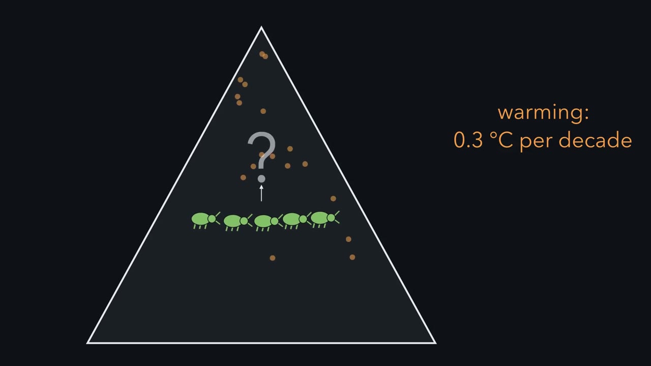 ▶ Watch The Climbing Line · 3:08
Read the transcript of “The Climbing Line”
Film transcript: The Climbing Line
A mountain warms by 0.3 °C each decade. How far uphill must the beetles' range shift, to stay as cool as before? Picture the slope as stacked bands of temperature, warm at the bottom and cool at the top. The gold line is an isotherm, a line of equal temperature. This beetle lives only where it is cool enough. So the gold line marks the lower edge of its range, the warm edge. Now warm the whole mountain. Every band slides upward, and the gold line climbs with them. The beetle's climate is on the move. How fast does the line climb? That depends on how quickly air cools with height, a slope's lapse rate. Here it cools 0.6 °C every 100 metres. Divide the warming rate by the lapse rate.
The result is the climate velocity, the speed of the isotherm. On this slope, it is fifty metres uphill each decade. Now let the population move, as beetles settle higher and low ones die out. The green band climbs, but slower than the gold line. The red bracket between band and line is the gap. Each decade the line pulls further ahead. If the beetles started in step, the gap is the difference in speeds, times the time. So moving is not the same as keeping up. A range keeps up only by moving as fast as its isotherm. Now set a flat plain beside it. There, temperature changes toward the pole, and far more slowly with distance. So on the flat, how far toward the pole gives the same cooling as one metre uphill?
A metre, a hundred metres, or about a kilometre? In one European example, about a kilometre and a half. A short climb buys the cooling of a long journey. The exchange rate varies by place. So raw distances cannot say which shift kept up. Each shift is judged against its own isotherm, on its own slope or plain. A 2011 synthesis pooled many studies of land species. The median shifts were about 17 kilometres poleward and 11 metres uphill each decade. But the medians hide wide variation. Some species ran ahead of their isotherm, and many lagged behind it. One last warning. For a forest beetle, clearing the lower slope can lift the range's bottom edge, whatever the temperature does.
A shift shows change, not its cause. A range keeps up only by moving as fast as its isotherm.
From the film
- Warming moves an isotherm, a line of equal temperature, poleward and uphill.
- The isotherm's speed, the climate velocity, is the warming rate divided by how fast temperature changes across the land.
- On a slope cooling 0.6 C per 100 m, warming of 0.3 C per decade moves the isotherm about 50 m uphill per decade.
- In one European example, one metre uphill gives the cooling of about 1.5 km poleward; the exchange rate varies by place, so each shift is compared with its own isotherm.
- A range keeps up only by moving as fast as its isotherm; a shift shows change, not its cause.
Eleven metres uphill a decade looks feeble beside 17 kilometres poleward, the first film’s two medians. Which shift kept up? Raw distances cannot say, because a species is racing its isotherm, not a distance.
The one idea. Under warming, a range keeps up only by moving as fast as its isotherm, a line of equal temperature. The isotherm’s speed, the climate velocity, is the warming rate divided by how fast temperature changes across the land; on a mountain that rate is the lapse rate, the drop in temperature with height. If a range started in step, its lag is the difference in speeds multiplied by the time.
Scope: this is a model for a range edge set mainly by temperature, under steady warming and lapse rate. Ranges move through colonization and local loss over generations, not by animals walking, and a population can also persist without moving, through plasticity, evolution or cool pockets of habitat. A growing gap shows that something changed, not what caused it.
Moving: species shift poleward and uphill
A species’ range is the area where its populations live and reproduce. Temperature falls with latitude and elevation (climate and biomes), so if temperature sets the edge of a species’ tolerable conditions, part of its niche, the edge should follow its isotherm poleward and uphill.
How was the movement shown? I-Ching Chen, Chris D. Thomas and colleagues pooled published range shifts of terrestrial species in a meta-analysis, a statistical synthesis of results from many studies (Science, 2011). Each data point was the mean shift of one taxonomic group in one region. Shifts were greatest in studies whose regions had warmed most. That match between shift and warming is what links the shifts to climate here, though it is a correlation across studies.
Did the shifts keep up? In one European example the two medians track about the same temperature change, roughly 0.07 C per decade (Going deeper), so the medians alone cannot answer. Setting each study’s shift against its own region’s warming gave the verdict: poleward shifts on average roughly kept pace, but most uphill shifts fell short of what the warming predicted.
The pattern holds in the sea too. In BioShifts, a global database of 30,534 range-shift records, Lenoir and colleagues (2020) found marine species moving poleward about six times faster than terrestrial ones. Land species lagged further behind their shifting isotherms, and human activities hindered their tracking of isotherm shifts in latitude.
Keeping pace: climate velocity on a mountain
How far behind its isotherm is a species on a slope? The first film’s rule:
In words The isotherm's climb each decade is the decade's warming divided by the lapse rate.
- isotherm shift per decade“isotherm shift”
- how far uphill the isotherm moves in ten yearsm per decade
- warming per decade“warming”
- how much the air warms in ten yearsC per decade
- temperature drop per metre of elevation“lapse rate”
- cooling per metre of heightC per m
Sanity check Keep the 100 m in the units: 0.3 / 0.6 is 0.5 of a 100-m step, so 50 m, not 0.5 m. A steeper lapse rate means a shorter climb.
Try one number
Predict. On the first film’s slope, whose round figures are invented, the isotherm climbs 50 m per decade. A species moves uphill at Chen and colleagues’ terrestrial median, 11.0 m per decade, the one rate here from data, and starts in step with its isotherm. What share of the isotherm’s shift does it match, and how far behind is it after 30 years?
Check your prediction
- Share. 11.0 / 50 = 0.22, or 22% of the isotherm’s shift.
- Lag over 30 years. Over 3 decades the isotherm moves 3 x 50 = 150 m; the species moves 3 x 11.0 = 33 m. The species ends up 117 m below the elevation that now has its former temperature.
Beyond the box’s assumptions (constant warming and lapse rate, a range set by temperature alone), the sum assumes a species that started in step and no road, farm or cliff in the way. A real lag could reflect slow dispersal, cues other than temperature, competitors or predators already upslope, or loss of forest, and a particular species could be far ahead of its isotherm or far behind it.
- Isotherm speed, (warming / lapse) x 100 m
- Share of isotherm’s shift matched
- Isotherm has moved
- Species edge has moved
- Lag behind the isotherm
In this sketch: constant warming and lapse rate, the species’ range is set by temperature alone, and nothing such as a road, a farm or a cliff blocks it. The mountain is not to scale and its starting elevation is not given. The default species rate, 11.0 m per decade, is the median of Chen and colleagues’ 2011 meta-analysis; the other numbers are invented round figures, and a particular species could be far ahead of or far behind the median.
Rule to keep: the isotherm moves (warming / lapse rate) metres per decade; a species that moves slower than that falls behind by the difference in rates each decade, and a real lag could reflect slow dispersal, cues other than temperature, competitors or predators already upslope, or loss of forest.
Why it matters. Species do not move together, so communities come apart and reassemble, and hosts and pathogens meet in places they had not shared before (Van Hemert and colleagues, 2014, on Arctic birds). Pecl and colleagues (Science, 2017) reviewed evidence that climate-driven redistribution is already altering the composition of communities and changes ecosystem functioning and human well-being, through food production, disease transmission and carbon storage.
A similar gap can open in phenology, the seasonal timing of life-cycle events, when a consumer and its food shift by different amounts; the second film follows one bird and its food.
Read the transcript of “Two Forests, One Bird”
Film transcript: Two Forests, One Bird
If a bird lays its eggs earlier every spring, is it keeping up? The first film measured a gap in space, between a species and its isotherm. This film measures a similar gap in time. The seasonal timing of life events is called phenology. Leafing, flowering, migration and egg laying are all phenology. As springs have warmed, many of these now come earlier.
Now one bird and its food. The gold curve is the caterpillar peak, the food supply. The green bar is when nestlings need feeding most. Here they start in step. Warm the springs. The gold peak slides earlier. The green bar slides earlier too, but by less. A red bracket can open between them. That gap is trophic mismatch.
Demand now peaks after the food peak has passed. So an earlier date, on its own, cannot show keeping up. Does mismatch cost birds? Christiaan Both and colleagues compared nine Dutch populations of the pied flycatcher. It winters in Africa and breeds in European woods. In some of the forests, caterpillars peaked early. In others they peaked late, and birds that bred early were still well timed. Where food peaked early, flycatcher numbers fell by about ninety percent over two decades. Where it peaked late, declines were weak at most. The early forests lost about nine pairs in every ten. Does that comparison prove that mismatch caused the loss?
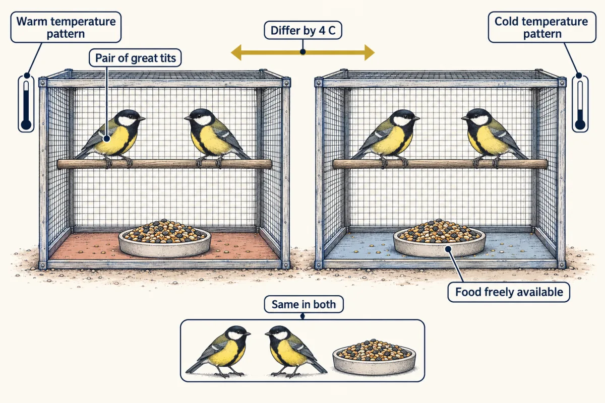
Not yet. It supports a cost of mismatch, but it compares sites. The forests were not assigned their caterpillar timing, so something else could differ between them. A second question. What tells a bird when to lay? In the field, warm springs bring early laying, but they also bring early food. The pattern alone cannot separate them. Marcel Visser and colleagues kept breeding pairs of great tits in climatized aviaries. Every aviary had food freely available. Only the temperature pattern differed, warm or cold. The warm aviaries generally laid earlier. With food unlimited, the authors read temperature as likely acting as a cue, a signal the birds respond to.
Each design answers its own question. A trend suggests a change. Testing it against chance and natural variation is detection. The forest comparison links food timing to decline, but sites can differ in other ways. The aviaries show temperature acting on laying, in great tits. Through all of it, the date alone never answered the question. What counted was the gap between the food and the family.
From the film
- Many spring events now come earlier, but interacting species often shift by different amounts, so an earlier date alone cannot show keeping up.
- Trophic mismatch is the offset between peak food and peak demand, such as nestlings in the nest; unequal shifts can open or widen it.
- In nine Dutch pied flycatcher populations, numbers fell about 90% over two decades where caterpillars peaked early, and weakly at most where they peaked late.
- That comparison across sites supports a cost of mismatch, but the forests were not assigned their food timing.
- In aviaries with food freely available, a warmer temperature pattern generally advanced great tits' laying, pointing to temperature as a likely cue.
Timing: phenology and mismatch
Besides the unassigned forests, the second film’s “not yet” has a second reason: Both, Visser and colleagues (Nature, 2006) measured the cross-site caterpillar peaks in a single year (Going deeper), so the contrast supports, but does not by itself establish, a causal effect of timing on population size.
A loss at the nest must also carry through to the number of adults before mismatch reaches demography.
Predict. In a great tit population, mismatch cuts the number of young that fledge, or leave the nest. Must the population shrink?
Check your prediction
Not necessarily. Visser and Gienapp (2019) describe great tits in which mismatch reduced the number of young that fledged, yet more of those young survived their first winter in years when few were produced, so population growth showed no detectable effect. That is density dependence: a rate, here first-winter survival, that changes with the number of animals, so a loss at the nest can be made up later. A mismatch has to be linked to population change in the data, not assumed.
Visser, Holleman and Caro (Proceedings of the Royal Society B, 2009) ran the aviaries for six years, with warm and cold patterns 4 C apart in the period that mattered, and the warm treatment advanced laying in five; the cue is the authors’ reading.
The other drivers: land, aliens, acid and nitrogen
These drivers act alongside warming and need not act solely through a moving isotherm, though cleared land can also alter local climate; attribution to warming tests those plausible for the response, place and period. Direct exploitation, such as fishing, hunting and logging, is another major driver that this lesson leaves aside.
Land use. Converting forest and grassland to farms, pasture and towns removes habitat outright; reviews, among them the IPBES global assessment (2019), name this habitat loss as the largest single driver of the decline in land biodiversity. Newbold and colleagues (Nature, 2015) modelled a global database of terrestrial assemblages and estimated that land use and related pressures have reduced within-sample species richness by an average of 13.6%, and by 76.5% in the worst-affected habitats. These are model estimates from sampled sites. Land use also acts with climate: in average elevational shifts from 43 study sites, Guo, Lenoir and Bonebrake (2018) found that forest loss in warmer regions tended to go with faster upslope movement, a correlation across sites consistent with the first film’s cleared lower slope. An uphill shift is not by itself proof that climate acted alone.
Species moved by people. An alien species is one moved by people beyond its native range (Blackburn and colleagues, 2014). Using IUCN Red List data, Bellard, Cassey and Blackburn (2016) found that alien species were the second most common threat associated with plant and vertebrate extinctions since 1500, and the most common for vertebrates. Impacts run through competition, predation, hybridisation and other mechanisms, and range from minimal to massive. New aliens keep arriving: more than a third of all recorded first records of established aliens fall in 1970 to 2014 (Seebens and colleagues, 2017), though a first record can lag the real introduction, so that curve tracks detection as well as arrival.
Ocean acidification. Carbon dioxide dissolving in seawater forms carbonic acid (the equilibria are in water and weak bonds):
CO2 + H2O ⇌ H2CO3 ⇌ H+ + HCO3-, and H+ + CO3 2- → HCO3-
Net: CO2 + H2O + CO3 2- → 2 HCO3-
In plain terms, the acid’s hydrogen ions lower pH and use up the carbonate that shells are built from, lowering the saturation state of calcium carbonate, which compares the calcium and carbonate in the water with the amounts at which calcium carbonate neither forms nor dissolves: above 1, forming the mineral is chemically favoured; below 1, unprotected calcium carbonate tends to dissolve. Organisms differ, and their calcification has no universal threshold at 1. Surface seawater stays alkaline, above pH 7, while this happens; “acidification” names the direction of change. Pooling 228 studies, Kroeker and colleagues (2013) found that acidification on average lowered calcification, growth and survival, with wide differences between groups. A later synthesis of 985 studies (Leung and colleagues, 2022) found many calcifiers, such as echinoderms, crustaceans and cephalopods, tolerant of near-future acidification, while corals, coccolithophores and calcifying algae appeared sensitive, and larvae were generally more sensitive than adults.
Predict. Ries, Cohen and McCorkle (Geology, 2009) held 18 species of benthic (sea-floor) calcifiers at controlled CO2 levels, the highest about ten times pre-industrial. Did every species calcify less?
Check your prediction
No. More than half calcified less, several calcified more and one did not respond (tally in the anecdote on the blue mussel): the same spread as the syntheses.
Nitrogen deposition. Burning fuel and making fertilizer put reactive nitrogen into the air, and it falls on distant land (nutrient cycling).
Predict. Nitrogen often limits plant growth. On Minnesota prairie, where ambient deposition was 6 kg N per hectare per year, what would adding 10 kg N per hectare per year more do to the number of plant species?
Check your prediction
It cut it. Christopher Clark and David Tilman (Nature, 2008) found that the addition reduced plant species number by 17% relative to controls. In a second experiment, species number had recovered a decade after additions stopped, but species abundances had not.
Why does a nutrient cut diversity? Added nitrogen tends to reinforce the dominance of a few species, and the resource they win differs between places: light in one grassland experiment, water in a semi-arid grassland. Soil acidification adds a further route, more so at high doses (all three in Going deeper). How species loss changes ecosystem processes is the subject of biodiversity and ecosystem function.
How strong is the attribution?
A gap says how far a species fell behind; attribution asks why. Keep three kinds of claim apart.
- Detection shows that a change happened beyond what chance or natural variation would produce, not what caused it.
- Attribution links the change to a cause and tests the alternatives. Attribution to human-caused warming takes two links: from the biological change to regional warming, then from regional warming to human causes (the IPCC’s wording is in Going deeper).
- Projection is what a model gives under a stated scenario of emissions or land use. It is a conditional result, not an observation of the future.
Rosenzweig and colleagues (Nature, 2008) found that continental-scale warming associated with observed changes in physical and biological systems could not be explained by natural climate variation alone. Their data were concentrated in Europe and North America, and the BioShifts range records are likewise biased toward the developed regions of the Northern Hemisphere, so global summaries describe a biased sample.
Each design answers its own question, as the second film showed. A manipulation that assigns the driver (aviary temperature, prairie nitrogen, seawater CO2) shows cause in that preparation but not why the field warmed; a comparison across sites is stronger than a single trend but can be confounded; a covariate-adjusted association, a statistical model that includes measured rival drivers such as warming and forest loss, can expose a confounder it measured but not one it did not. For any claim, ask five questions: what response was measured, what driver is proposed, what alternatives were tested, where the independent variation came from, and how large the uncertainty is. Decisions in conservation rest on those answers.
Design problem
At one site, a bird’s laying date has advanced 10 days over 30 years, while the peak of its caterpillar prey advanced 20 days. The population has fallen. What evidence would show that the growing mismatch caused the decline, and what would it take to connect that to human-caused warming?
Saved in this browser only.
One way to do it
First, the arithmetic: the prey peak moved 20 - 10 = 10 days more than laying, so the offset changed by 10 days and the bird matched half its prey’s shift. Laying date stands in for peak demand only if the time from laying to hungry nestlings stays the same. Whether the change created a harmful mismatch depends on how well timed the birds were at the start, and much else changed in 30 years.
- Replicate across populations. Compare many populations whose prey peaks differ in timing, as Both and colleagues did for Dutch pied flycatchers. If mismatch matters, decline should be steepest where the gap is largest.
- Measure every year. Record the prey peak and laying dates annually, not in a single year.
- Measure vital rates, the rates of birth and survival. Track fecundity (young produced), nestling and juvenile survival, and adult survival, including on migration and in winter. Mismatch should show up mainly in breeding success and the survival of young. If a fall in adult survival on the wintering grounds explains most of the decline, mismatch is unlikely to be the main cause, though carry-over effects, where one season’s conditions affect the next, can blur that line.
- Test alternatives. Measure habitat change at the breeding site, conditions on the wintering grounds and along the route, predators and disease.
- Experiment where possible. Supplementary feeding after the natural peak could test whether food timing limits breeding success.
Even a convincing case that mismatch drove the decline attributes it to timing, not yet to human-caused warming; that needs evidence that the local spring warming is itself attributable to human forcing.
Going deeper
One metre uphill, in kilometres poleward
One illustrative pair of stations: in 1991–2020 climate normals, the annual mean is 15.8 C at Rome Ciampino and 7.9 C at Stockholm, about 17.5 degrees of latitude (roughly 1,950 km) farther north, about 0.4 C per 100 km. With the first film’s lapse rate of 0.6 C per 100 m, one metre uphill matches about 1.5 km poleward there. This is not a general conversion: gradients differ between regions, seasons and stations, so each study should use its own local gradient. On these figures Chen and colleagues’ two medians each track roughly 0.07 C per decade.
The two links of attribution
In the IPCC’s 2007 assessment (AR4; later assessments have updated the wording), “joint attribution” links a biological change to regional climate change and then links part of that climate change to human causes, while assessing plausible alternative explanations.
How the flycatcher food peaks were measured
The pied flycatcher is Ficedula hypoleuca. The comparison was observational: the cross-site caterpillar peaks were measured in one year, 2003, and a second index of food timing came from the share of great tits laying second broods in 1985 to 1990.
Why nitrogen cuts diversity: light, water and soil
In experimental grassland plant communities, Hautier, Niklaus and Hector (Science, 2009) added light to the understory and prevented the loss caused by fertilization, which implicates competition for light. In a semi-arid grassland in China, Li and colleagues (2024) found that adding water prevented species loss under nitrogen alone or warming alone, but only partly when both were combined. Nitrogen also acidifies soil, and in a field experiment and meta-analysis Namuhan and colleagues (2024) found that toxic manganese and aluminium ions contribute to the loss, more so at high nitrogen doses. Neither the light nor the water mechanism is universal, and they are not the only ones.
Your notes
Select any text in the lesson to highlight it or add a note to it. Your highlights and notes are saved in this browser and collected in your notebook.
This browser is not letting the site save anything (a private window or strict privacy settings), so highlights and notes will be lost when you leave the page.
How we measure it
Range-shift meta-analysis
Published changes in range position from many studies are pooled and analysed together, keeping latitude and elevation apart. It gives medians and spreads across species and can test whether shifts are larger where warming was larger, but it inherits the geographic and taxonomic gaps of the studies it pools.
Climatized-aviary temperature manipulation
Breeding birds are housed under controlled temperature patterns with food available, and laying dates are compared between treatments. It tests whether temperature itself changes timing, separating that effect from food and other variables that go with warm springs in the field.
Factorial nutrient-addition and resource-rescue experiments
Plots receive added nitrogen or not, and each of those groups is split into plots with and without a second treatment that restores a resource suspected of being limiting (light to the understory, or water). If the restored resource prevents the species loss, that resource competition is implicated in that system.
Buoyant weighing of calcifiers
An organism is weighed underwater before and after an exposure, and the change in its buoyant weight estimates how much calcium carbonate it gained or lost. It lets many species be compared under the same seawater chemistry.
Practice questions on this lesson (3) → MCAT-style, original, each with an explanation
Where this lesson fits
Before thisReview first
- Climate, Biomes and Environmental VariationThis course · Lesson 11
You need the fall of temperature with latitude and height from there to work out how an isotherm moves.
- Distributions, Niches and TolerancesThis course · Lesson 12
Here a range edge follows temperature tolerance, an idea built in that lesson.
- Nutrient CyclingThis course · Lesson 22
Nitrogen deposition here assumes you know how reactive nitrogen moves through ecosystems.
After thisStudy next
- Conservation and RestorationThis course · Lesson 25
It uses range shifts and other drivers of loss to decide what to protect and restore.
- Integrative Evidence WorkshopThis course · Lesson 26
It asks you to judge what evidence can show about a cause, as attribution does here.
Suggested by an AI model from the lessons themselves, then checked. How we use AI
Finish line
Test yourself
8 questions
Practice and MCAT-style, with explained answers.
Next · Lesson 25
Conservation and Restoration
In 1995, eight female pumas from Texas were released into the Florida panther population. What did that change, and how would you know?
Continue →