Ecology and Evolution · Unit 3: Environments and populations
Distributions, Niches and Tolerances
Rewritten on : new text, flashcards and film. Your notes and highlights stay, but the text around them may have moved.
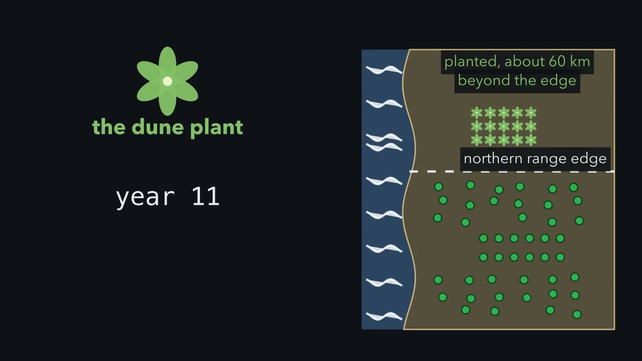
A dune plant was planted 60 km past its own range edge, and the planted population more than tripled. So what was stopping it?
Pause when the reading reaches a film, and offer to play it. Saved on this device.
Watch the film now, or keep listening
Builds on:Climate, Biomes and Environmental VariationNatural Selection in Ecological ContextWhy these?
 ▶ Watch Where It Can Live, Where It Is · 3:21
Read the transcript of “Where It Can Live, Where It Is”
Film transcript: Where It Can Live, Where It Is
A dune plant was planted about sixty kilometres past the northern edge of its range. The planted population more than tripled. If it can live there, why was it never there? To answer, keep two things apart. One is the set of conditions a species can live in. The other is the map of where it is found. Draw the conditions first. Put temperature on one axis and soil moisture on the other. Each sampled spot becomes a point, and one place can give several. Now ask one question at each point. Count a local population once a year, with no newcomers. By what factor does it multiply that year? Ecologists call that factor lambda. Years differ, so lambda changes from year to year.
The test uses the long-run lambda, good and bad years together. One good summer does not count. Where long-run lambda is at least one, the population replaces itself without immigrants. That region of conditions is the niche, drawn as a teal box.
Now turn to the map. Shade every stretch of coast whose conditions fall inside the box. That teal shading is where the species could live. Then add the places where the species is actually found, as dark green dots. The dots and the shading do not match. Picture a teal stretch with no dots. Its conditions are inside the niche. Nothing has arrived to start a population. So absence alone does not mark the edge of a niche. A species can be missing from a good place because it never got there. Now the other mismatch. A plant turns up at one site in every survey, year after year. Is that site inside its niche?
Not necessarily. Here deaths outnumber births, so lambda is below one. Seeds arriving from a neighbouring site replace the dead every year. Cut off the arriving seeds, and the plants dwindle away. A population like this, kept going by immigrants, is called a sink. So presence alone does not mark the niche either. A map shows only where the species is found. Spotting sinks takes counts of births, deaths and immigrants. Other species change lambda too. A competitor or an enemy can push it down. A helper can push it up. Back to the dune plant. Its planted population grew past the edge. So, at least at that site, the edge is not where the plant fails.
A niche is where long-run lambda is at least one without immigrants. A map shows only where the species is found.
From the film
- A niche is the set of conditions in which the long-run lambda, across good and bad years with no immigrants, is at least 1.
- Niche space is a space of conditions; the map shows the places where the species is found.
- A species can be missing from a place inside its niche because it has never reached it.
- A sink population lives outside the niche and is kept going by immigrants, so presence alone does not mark the niche.
A range map blurs three things: the conditions a species can live in, the other species it meets, and the places it has reached.
The one idea. Count a local population once a year. Next year’s count is this year’s multiplied by λ (lambda), the factor its own births and deaths produce that year, plus any immigrants, I: Nnext = λ·N + I. A species’ niche is the set of conditions in which the long-run λ, taken across good and bad years with no immigrants, is at least 1. A map adds two mismatches: suitable places never reached, and places outside the niche where immigrants keep a population going. Other species move λ, down (competitors, enemies) or up (helpers).
Scope, for every λ in this lesson: one species at one site, counted as a single number and closed except for immigrants (a stage-structured model, used in the transplant studies, does the same bookkeeping stage by stage); λ is judged while the population is sparse; chance births and deaths in very small populations, which can end one even at λ = 1, are set aside, as is evolution at the edge over the length of an experiment.
The bookkeeping behind a map
The first film drew the niche; here is its bookkeeping. λ, the finite rate of increase, sums up survival, growth and reproduction across the whole life cycle, the vital rates from life histories.
In words Next year's count equals this year's count times lambda, plus the immigrants that arrive.
- N“N”
- plants at the site this yearplants
- Nnext“N next”
- plants at the site one year laterplants
- λ“lambda”
- the finite rate of increase: the factor the residents multiply by that year, without immigrantsnone (a factor per one-year step)
- I“I”
- new plants arriving from elsewhere that yearplants
Sanity check With I = 0 the population grows if λ is above 1 and shrinks if it is below 1. With N = 0 and I = 0 it stays at zero.
Try one number
λ = 0.8 every year, with 20 new plants arriving a year: the count levels off where losses match arrivals, at 20 / (1 − 0.8) = 100 plants, present in every survey. Cut off the arrivals and it falls toward zero.
The niche test uses long-run λ with I = 0 because a run of good years can hide a rare bad one (Going deeper).
G. Evelyn Hutchinson gave the niche this form in 1957: with n axes (temperature, soil moisture, salt, the size of food items) it is an n-dimensional hypervolume in niche space, while geographic space is the map. Conditions vary with latitude, altitude and microclimate (climate and biomes), so one patch of niche space can map onto scattered places, and one place can hold several microclimates.
The card’s two cases are the first film’s two mismatches: N = 0 with I = 0 is a place never reached, and the steady 100 plants at λ = 0.8 are a sink population.
Fundamental and realized niches
Hutchinson split the niche in two. The fundamental niche is the set of conditions in which a species can persist with no competitors or enemies present (fine print in Going deeper). The realized niche is the set of conditions it occupies when other species are present. Competitors and enemies usually make it a smaller part of the fundamental niche; helpers can extend it past it.
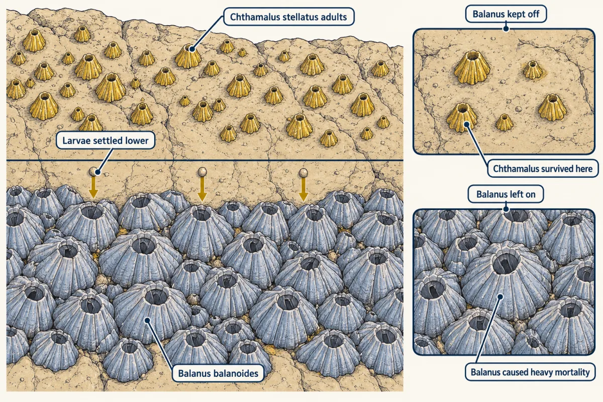
Joseph Connell’s classic field case, published in 1961, comes from the rocky shore at Millport on the Isle of Cumbrae, Scotland. Adults of the barnacle Chthamalus stellatus lived in a band high on the rocks, above the larger Balanus balanoides. Yet Chthamalus larvae settled lower.
Predict. Something removes the Chthamalus that settle below the adult band. Name two things that could do it, and an experiment that would tell them apart.
Check your prediction
Low-shore conditions, or the competitor Balanus: keep Balanus off some patches of lower rock and leave it on others. Connell did; the figure below shows what he found.
So a competitor left the lower part of the Chthamalus fundamental niche unoccupied. Connell attributed the upper limits mainly to heat and drying, with Chthamalus the more tolerant (competition has the experiment in full).
Helpers work the other way. A shrub that shades seedlings, or a mussel bed that holds water at low tide, raises λ and can let a species persist in conditions it cannot tolerate alone. If the fundamental niche is defined before any interaction, the realized niche then reaches past the fundamental one, so “the realized niche is always smaller” has exceptions (a framing some ecologists dispute).
Species distribution models, fitted to the climates of places where a species has been recorded, describe the map, sinks and gaps included: occupied conditions plus accessibility, closer to the realized niche filtered by dispersal than to the fundamental niche.
Tolerance: one piece of λ at a time
Rearing individuals in the laboratory at several constant temperatures and recording a named response gives a thermal performance curve. For a rate such as development, it rises from zero at Tmin, peaks at Topt and falls to zero at Tmax; survival curves are often flat across middle temperatures. The fall at high temperature has several causes, among them proteins losing their folded, active shape, as in enzyme action.
Every value belongs to its response: for development, Tmin and Tmax are where that rate reaches zero, not necessarily lethal temperatures. If a step every individual must pass through, such as development to adulthood, stops at some temperature, the life cycle cannot be completed there and λ is below 1 whatever the other rates do. Short of that, λ has to be worked out from the whole life cycle.
Predict. Development rate and survival both fall at extreme temperatures. Across moths and butterflies, which would you expect to limit performance at the cold end, and which at the hot end?
Check your prediction
In a 2024 synthesis of laboratory data sets for Lepidoptera, Mariana Abarca and colleagues found that development rate generally limited performance at the cold end and survival at the hot end. So different rates set the two ends; Going deeper works a breadth from both.
A laboratory breadth is not a range boundary: a moth in the field can shelter in shade, and its distribution also depends on host plants, enemies and dispersal. A chamber measures one piece of λ; to learn whether a whole population can replace itself past an edge, you have to plant it there, as the second film does.
Read the transcript of “Planting Past the Edge”
Film transcript: Planting Past the Edge
A plant's range ends at a headland. Why does it stop there? Is it the cold, the neighbours, or seeds never getting there? The first film drew a niche as the conditions where lambda stays at or above one without immigrants. Now we test an edge directly. Each answer is a different kind of limit.
Conditions make an abiotic limit. Other species make a biotic limit. Never arriving makes a dispersal limit. The direct test is to plant the species beyond the edge and follow it for years. But plant the same way inside the range too.
Transplanting itself is a shock, and a bad year can kill plants anywhere. Then split every site in two. On randomly chosen plots, clear away the neighbouring plants. On the others, leave them. Count survival, growth and seed production across the whole life cycle. From those, estimate lambda for every plot. One season's survival is not enough. First possible result.
Lambda beyond the edge stays at or above one, with or without neighbours. The species can live there. Seeds have not arrived, or have not recolonised empty patches. The dune plant looks like this case, though its neighbours were never cleared. Planted beyond its northern edge, the population more than tripled in twelve to fourteen years. Second result. Beyond the edge, lambda falls below one only on plots where neighbours remain. Cleared plots do fine. Other species are setting the limit. Third result. The plots inside the range grow. Beyond the edge, plots shrink whether or not neighbours were cleared. What does that implicate?
The conditions beyond the edge. Climate is a strong candidate. But herbivores, pathogens or missing soil partners need their own tests first. One more result. Every plot fails, inside the range as well as beyond it. Then the test cannot single out the edge.
Handling, the seed or a bad year may be to blame. Check them, then repeat the study. So here is the reading rule. Compare lambda beyond the edge with lambda inside the range, on plots with and without neighbours. That comparison separates access, neighbours and conditions beyond the edge. A map of where the species grows cannot do it on its own. Plant beyond the edge, with the same planting inside, and measure lambda. Where it replaces itself beyond the edge, the range stops short of the niche.
From the film
- A range edge can be set by conditions, by other species, or by access: the species not arriving or not recolonising.
- Planting beyond the edge, with the same planting inside the range, tests which; if the inside plantings fail too, handling, the seed or a bad year may be to blame, and the test cannot single out the edge.
- Clearing neighbours on random plots separates the neighbours' net effect from a limit set by conditions.
- Lambda over the whole life cycle, not one measure such as first-year survival, decides whether a population can persist.
- The dune plant grew beyond its northern edge, so at that site the edge was not where the plant fails; its neighbours were not tested.
Testing a range edge
Amy Angert and Douglas Schemske grew two California monkeyflowers, Mimulus cardinalis of low elevations and M. lewisii of high ones, in gardens inside and beyond each species’ elevation range. Each had zero or near-zero fitness beyond its limits, which fits niche limits, but elevation changes many conditions at once, so temperature cannot be separated from the rest.
How often is a range edge a niche edge? In 2014 Anna Hargreaves, Karen Samis and Christopher Eckert meta-analysed 111 transplant tests beyond the range; in three quarters, performance fell beyond the edge.
Predict. Nnext = λ·N + I allows one kind of edge the second film did not show. What is it?
Check your prediction
A range that runs past the niche limit, its edge populations sinks (λ below 1, I above 0). In a transplant, plants fail even just inside the edge. The review found all three. In 46% of tests the range limit sat at a niche limit. In 26%, mostly latitudinal or longitudinal limits, transplants sustained themselves beyond the range, consistent with dispersal limitation (λ at least 1, N = 0). In 23%, all at elevation limits, the range ran past the niche limit. The shares do not add to 100%.
The opening dune plant, Camissoniopsis cheiranthifolia, is the second film’s first result; Regan Cross and Christopher Eckert revisited it 12 to 14 years after planting. Exactly tripling in that time means multiplying by about 1.08 to 1.10 a year on average, more than tripling a little more: a species can sit just above replacement and still be missing (a rough illustration, not a measured long-run λ). They inferred that limits on local dispersal had likely contributed to the edge. Later surveys by Eckert’s group found that colonisation of empty dune patches falls toward the limit, where suitable habitat is scarcer and fewer plants grow nearby, so the edge may be held by a balance of colonisation and local extinction (empty patches colonised more slowly than occupied ones die out) rather than by seeds never arriving. One site shows the edge is not where the species fails there, not that every dune farther north is suitable. See spatial populations for movement between populations and global change for edges shifting under warming.
Design problem
Take the second film’s test of a range edge at a headland. What would you add before trusting its answer?
Saved in this browser only.
One way to do it
Keep the film’s plan and add:
- Seed from several source populations, so no one population decides the result, plus seed and sites from the range edge itself, as the 2014 review stressed.
- Several years of survival, growth and seed production, combined in a stage-structured model (one that tracks seedlings, juveniles and adults separately) to estimate long-run λ for each site and treatment.
- The landowner’s permission and often agency permits, sites that can be monitored, and removal of plants at the end if required, because a species that thrives there could spread as a new invader.
Read λ as the film does. Where it falls below 1 beyond the edge with and without neighbours, climate is a strong candidate, but herbivores, pathogens or missing soil partners need their own tests before the limit is called abiotic.
Going deeper
Why λ has to be a long-run rate
Predict. At one site λ alternates between 1.5 in good years and 0.6 in bad ones, an average of 1.05. Does the population grow?
Check your prediction
No. Each pair of years multiplies it by 1.5 × 0.6 = 0.9, so for a single count like this the long-run λ is the geometric mean, √0.9 ≈ 0.95, and 100 plants fall to about 12 in 40 years. One rare bad year does the same: λ = 1.1 for nine years and 0.3 in the tenth averages 1.02, but the long-run λ is about 0.97. Most transplants run a few years at a few sites, so rare lethal years and long-term adaptation at the edge are hard to capture.
Fine print on the fundamental niche
In the fundamental niche, the species’ food and any partner it cannot live without are assumed present. Hutchinson framed it in terms of competitors. Some treatments add biotic axes, such as the density of a predator, but the fundamental niche is usually drawn on physical conditions and resources.
Worked problem: a performance breadth from development and survival
The 2024 synthesis by Mariana Abarca and colleagues used 46 laboratory data sets from 26 species of Lepidoptera. They combined the two rates:
P = D x S (D = development rate, S = survival, each scaled to its own maximum)
The numbers are invented for teaching. A moth is reared at three temperatures. Survival peaked at a cooler temperature not shown, so S is below 1 at all three.
| Temperature | D | S |
|---|---|---|
| 20 degrees C | 0.50 | 0.80 |
| 25 degrees C | 1.00 | 0.60 |
| 30 degrees C | 0.80 | 0.20 |
Assume P changes in a straight line between treatments, do not extrapolate beyond 20 or 30 degrees C, and call the acceptable range P of at least 0.50 (the threshold Abarca’s group used, an operational choice).
- Compute P. 0.50 x 0.80 = 0.40 at 20 degrees C; 1.00 x 0.60 = 0.60 at 25; 0.80 x 0.20 = 0.16 at 30. The best tested temperature is 25 degrees C. The true peak could lie between treatments.
- Lower crossing. P must rise 0.10 of the 0.20 it gains from 20 to 25, half the way: 20 + (0.50 - 0.40)/(0.60 - 0.40) x 5 = 22.5 degrees C.
- Upper crossing. 25 + (0.60 - 0.50)/(0.60 - 0.16) x 5 = 25 + 1.14 = 26.14 degrees C.
- Breadth. 26.14 - 22.5 = 3.64 degrees C.
- Which rate limits each end? At 20 degrees C survival is high and development slow, so development limits the cold end. At 30 degrees C development is still fairly fast but survival has collapsed, so survival limits the hot end.
- D x S = P at 20 / 25 / 30 °C
- 0.40 / 0.60 / 0.16
- Lower crossing
- 22.50 °C
- Upper crossing
- 26.14 °C
- Breadth
- 3.64 °C
In this sketch: invented data for a moth at three constant temperatures, D and S each scaled to their own maximum, straight lines between treatments, no extrapolation beyond 20 and 30 °C. P leaves out fecundity, so it is not lambda; a crossing is not a lethal limit or a range boundary.
Rule to keep: the tolerance interval is where the combined response stays above a threshold you chose, found by interpolation inside the tested range, and the two ends can be limited by different rates.
P leaves out fecundity, so it is not lambda. The crossings are not lethal limits, and they are not a range boundary.
Field experiment on competition: the Welk study
Welk and colleagues grew 14 perennial grassland species in nine German botanical gardens, with a sown competitor grass, Festuca rubra, present or absent and molluscs excluded or not, in a fully crossed design. In their model, competition reduced the perennials’ aboveground biomass by 40.8% overall. Survival also declined as precipitation fell across the gardens, but climate varied among gardens rather than being assigned at random, so that part is an association.
Names and word history
Hutchinson did not coin the word niche: Joseph Grinnell used it in 1917 for a bird’s habitat and habits, and Charles Elton in 1927 for an animal’s place in a food web. The Millport barnacles are now identified as C. montagui, a separate species split from C. stellatus after Connell’s work, and Balanus balanoides is now Semibalanus balanoides.
Your notes
Select any text in the lesson to highlight it or add a note to it. Your highlights and notes are saved in this browser and collected in your notebook.
This browser is not letting the site save anything (a private window or strict privacy settings), so highlights and notes will be lost when you leave the page.
How we measure it
Transplants beyond the range, with within-range controls
Individuals or seeds are planted inside the range, at the edge and beyond it, with the same handling at every site. If only the beyond-range plantings fail, conditions there are implicated; if all fail, the test cannot single out the edge, and handling, planting material or a bad year may be to blame.
Neighbour removal and exclosure experiments
Competitors are cleared, or herbivores fenced out, on randomly chosen plots and left on others. Comparing the two estimates the net effect of those species on performance at a site, including any effect they have on physical conditions such as shade or soil moisture.
Thermal performance assays
Individuals are reared at several constant temperatures and a named response, such as development rate or survival, is measured at each. The curve that results shows where that response peaks and where it falls to zero.
Stage-structured matrix population models
Survival, growth and reproduction measured at each life stage are combined into a matrix that steps the number in each stage forward one year. If the same matrix holds every year, its dominant eigenvalue is the long-run lambda, the finite rate of increase per year; when years differ, long-run lambda is estimated from the sequence of yearly matrices. A long-run lambda of 1 or more, without immigrants, means the population can replace itself under those conditions.
Practice questions on this lesson (3) → MCAT-style, original, each with an explanation
Where this lesson fits
Before thisReview first
- Climate, Biomes and Environmental VariationThis course · Lesson 11
You need how conditions vary with latitude, altitude and microclimate to see why one niche maps onto scattered places.
- Natural Selection in Ecological ContextThis course · Lesson 3
This lesson sets aside evolution at the edge, so you should already know selection in its ecological setting.
After thisStudy next
- Population Growth and RegulationThis course · Lesson 14
It uses N_next = λN and the sparse-population rate to ask what regulates a population.
- Movement and Spatial PopulationsThis course · Lesson 15
It takes up the colonisation and local extinction balance that may hold a range edge and the sinks fed by immigrants.
- CompetitionThis course · Lesson 16
It works out how a competitor shrinks the realized niche, which the Connell barnacles only introduce.
Elsewhere on the siteFilms, simulations and method films in other courses
- Grow a population, then add limitsSimulation · Biology
Adding limits to a growing population shows how conditions can stop the replacement rate from staying above one.
- Follow the Energy ArrowsFilm · Life Science
It is not a match, so ignore.
Suggested by an AI model from the lessons themselves, then checked. How we use AI
Finish line
Test yourself
8 questions
Practice and MCAT-style, with explained answers.
Next · Lesson 13
Demography and Survivorship
Only 10 of 100 newborn females live to age 3. Can the cohort still more than replace itself?
Continue →