Ecology and Evolution · Unit 2: Genomes, development and diversification
New to this? Review it at high school level: Variation and Survival
Life Histories and Evolutionary Trade-offs
Rewritten on : new text, flashcards and film. Your notes and highlights stay, but the text around them may have moved.
If breeding can cost a bird its future, why do birds that lay more eggs often survive better from one year to the next?
Pause when the reading reaches a film, and offer to play it. Saved on this device.
Watch the film now, or keep listening
Builds on:Natural Selection in Ecological ContextHow to Test an Evolutionary ExplanationWhy these?
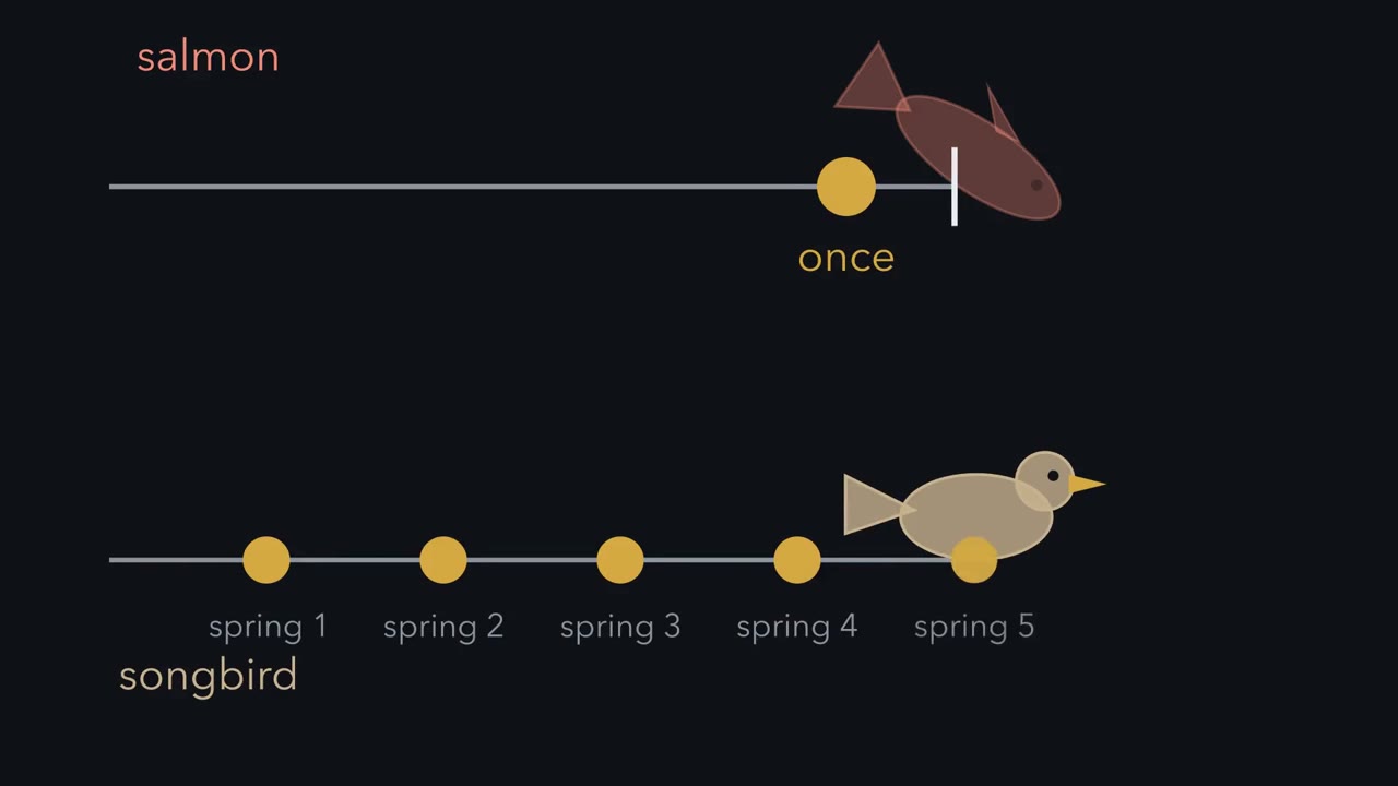 ▶ Watch One Budget, Many Uses · 3:18
Read the transcript of “One Budget, Many Uses”
Film transcript: One Budget, Many Uses
A salmon swims upriver, spawns once, and dies. A songbird nests every spring for years. Both are shaped by natural selection. So how can both strategies be right? Start with one bird in one season. Treat what it takes in and can use as one fixed budget. That budget must pay for four uses.
Upkeep, meaning maintenance and repair. Storage. And reproduction. Lump the first three together as self, in teal. Reproduction stays gold. For this one bird, gold plus teal always equals the intake. So more gold means less teal. That negative link is a trade-off.
Two classic trade-offs live on this line. First, current against future reproduction: what a parent spends on this year's young is not spent on itself. Second, number against size of offspring. A fixed amount put into a clutch can make many small eggs, or a few large ones. Picture two birds with the same intake. One pours most of it into this year's brood. The other keeps more for itself. Each sits at one point on the line, its split.
Selection acts on that split. It favours whichever split leaves the most descendants. Which split wins depends on who dies at what age. Picture two worlds. In the first, adults rarely survive the winter, but their young survive well. In the second, adults usually survive, while many young die, or their survival swings from year to year. Here is a question for you. In the first world, adults rarely live to breed again. Does that lower or raise the extra young one big bout needs to pay?
It lowers it. Holding back buys a future that rarely comes. So putting more into this year's bout can pay, as in the salmon. How far still depends on how extra effort changes breeding and survival. In the second world, teal buys more breeding seasons. Holding back to breed again can pay, as in the songbird. That is why no organism can grow fast, breed early, make many large offspring and live long all at once. Salmon and songbird follow one rule in different worlds. One intake, one split.
Selection picks the split that leaves the most descendants where that animal lives. There is one catch. So far every bird had the same intake. Real animals do not all take in the same amount. Hold that thought, because it changes what real data show.
From the film
- Treat what an individual takes in and can use as one budget, split among growth, upkeep, storage and reproduction.
- For one individual with a given budget, more to reproduction leaves less for itself: that negative link is a trade-off.
- Two classic trade-offs: this year's young against the parent's own future, and many small offspring against a few large ones.
- Selection acts on the split, favouring whichever split leaves the most descendants, given who dies at what age.
- Low adult survival lowers the extra young one big bout needs to pay, so putting more into this year's bout can pay; how far still depends on how extra effort changes breeding and survival. Where adults survive well, or young survive poorly, holding back to breed again can pay.
The first film split one bird’s budget and left out two things: how large an edge breeding once needs, and that individuals differ in what they take in.
The one idea. What an individual takes in sets the size of its budget; how it splits that budget among growth, upkeep, storage and reproduction is where trade-offs live; and selection favours whichever split leaves the most descendants, given who dies at what age. Because individuals differ in what they take in, a natural correlation can hide a trade-off; changing breeding effort at random is the stronger test.
Scope: allocation within individuals of one population, with energy and nutrients treated as one budget. Some costs run through particular nutrients, and a manipulation can show that extra breeding costs something without showing that one fixed budget is why (parents may forage harder), so “one budget” is a model to test, not a law. Random assignment balances parent quality only on average, so every treatment difference carries sampling uncertainty; and survival is only one place a cost can show (later breeding and offspring quality are others). Across species the logic gives a fast-slow pattern that need not hold among individuals.
An organism’s life history is its schedule: how fast it grows, when it first breeds, how many offspring it makes and how large they are, how often it breeds, and how long it lives. Fitness is an individual’s contribution to future generations relative to others in the same environment (selection in ecological context); lifetime reproductive success, the number of offspring an individual produces over its life (often counted as those that survive to breed), is one common measure. Acquisition is what an individual takes in and can use; allocation is how it splits that among uses. A trade-off is the negative link allocation creates: for one individual, more to one use leaves less for another. How heritable life-history traits are belongs to complex traits and GWAS.
Semelparity, iteroparity and the cost of reproduction
Semelparity is a single reproductive episode in a lifetime, usually followed by death: many annual plants, most Pacific salmon (genus Oncorhynchus), and century plants (Agave) are standard examples. Iteroparity is repeated reproduction, as in most birds, mammals and long-lived trees.
“A salmon dies because it spent everything on spawning” is a physiological description, not an evolutionary explanation. The evolutionary question is comparative: did individuals that put more into one bout leave more descendants than those that held some back to breed again?
Call c the chance that a newborn survives to breed (juvenile survival) and p the chance that an adult survives a year (adult survival). Take the simplest annual model: both types first breed at the same age, surviving young join the breeders by the next year, and crowding and ageing are left out. Each year a repeat breeder that makes b₂ young leaves c × b₂ young that will breed, plus itself with probability p. A once-breeder that makes b₁ young leaves c × b₁ and dies. They break even when c × b₁ = c × b₂ + p. Divide both sides by c:
b₁ − b₂ = p / c (the extra young a once-breeder needs to break even)
Predict. With c = 0.05 and p = 0.5, how many extra young must a once-breeder make in its single bout to break even? What if c rises to 0.5?
Check your prediction
p / c = 0.5 / 0.05 = 10 extra young. With c = 0.5 it is 0.5 / 0.5 = 1. This is Charnov and Schaffer’s (1973) survival-adjusted form of Cole’s (1954) result. A low bar does not by itself say how much to hold back; that also depends on the shape of the trade-off (Going deeper). The simple model leaves out year-to-year change: where the survival of young varies a lot from year to year, models predict that repeated breeding can also pay.
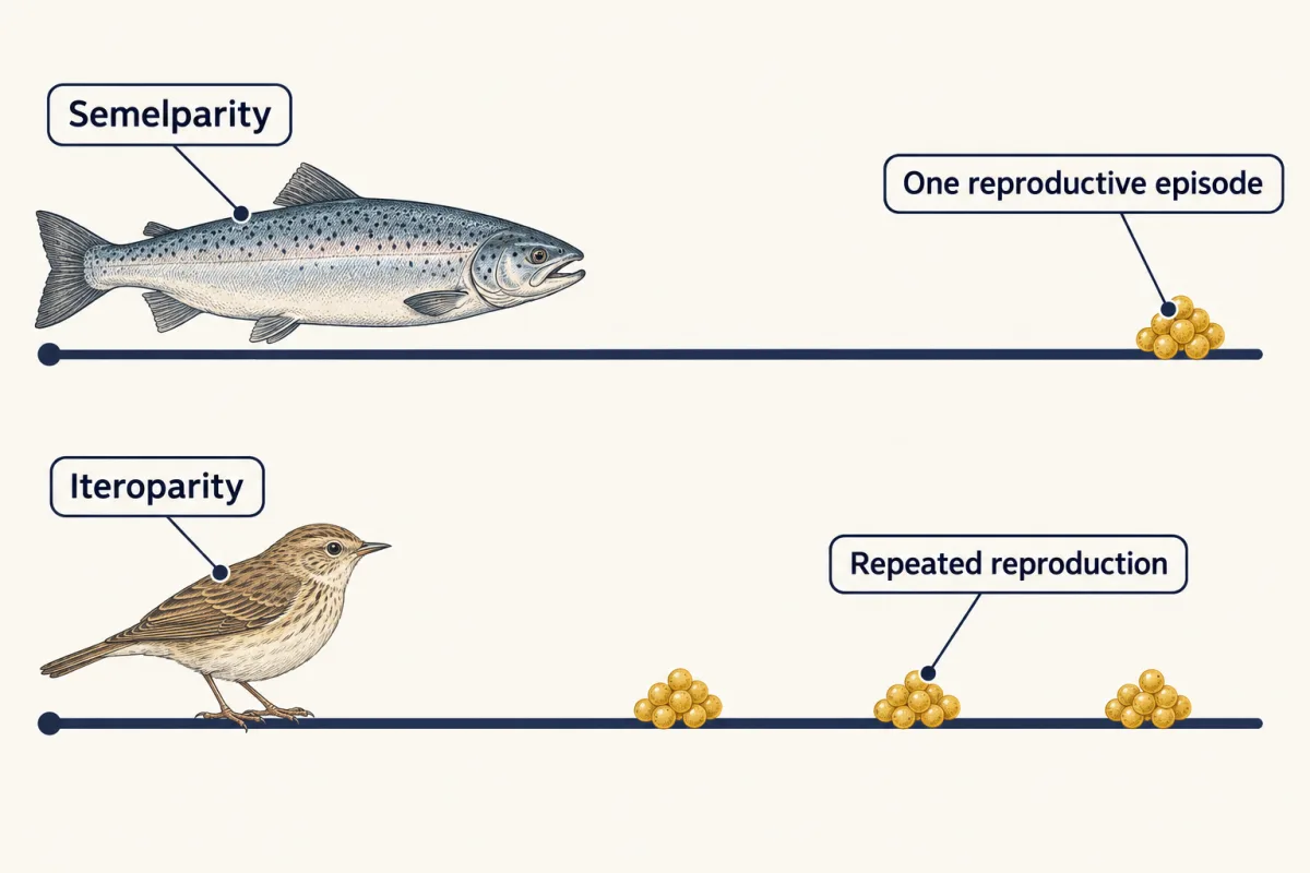
The cost of reproduction is the reduction in survival or future reproduction that follows from reproducing now. It is easy to assume and harder to show, because the cost need not run through a single shared budget. Dietary restriction lengthens life and lowers egg production in laboratory female Drosophila melanogaster, which looks like a classic trade-off. Grandison, Piper and Partridge (2009) added single nutrients back to the restricted diet. With methionine alone, fecundity (the number of eggs laid) rose to the fully fed level and lifespan did not shorten. In these flies, long life did not require low reproduction; the link ran through the balance of particular nutrients. The signalling pathways that sense such nutrients are in mTOR and AMPK. This is one species in the laboratory, and it gives no basis for any advice about human diet, fasting or supplements.
r and K, then the fast-slow continuum
r is the maximal intrinsic rate of increase, the rate at which a population grows per individual per unit time when nothing limits it. K is the carrying capacity, the population size the environment can sustain.
Robert MacArthur and E. O. Wilson introduced the terms r-selection and K-selection in 1967, and Eric Pianka’s 1970 paper in The American Naturalist listed what each should favour: early reproduction and little investment in each offspring where populations often grow freely (r-selection), and delayed reproduction and greater investment per offspring where populations sit near K (K-selection). He set semelparity against iteroparity in the same comparison, and in a 1979 commentary called the two ends of a spectrum, not a true dichotomy.
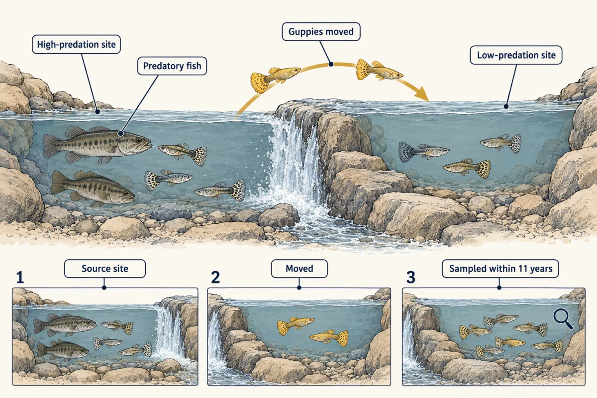
The scheme is best read as contrasting predictions, not a filing system. A species with early maturity and many small offspring has not thereby been shown to be under r-selection; other regimes can produce the same bundle. Field tests of particular causes have done better. In 1976 Endler moved guppies (Poecilia reticulata) in Trinidad from a high-predation site to a low-predation one in a tributary of the Aripo River. At the source site a large cichlid (Crenicichla alta) eats mostly adult guppies; at the new site a small killifish (Rivulus hartii) eats mostly juveniles, so the move shifted deaths from adults to young.
Predict. Which way should age at maturity and offspring size evolve?
Check your prediction
Later maturity and larger offspring. Reznick, Bryga and Endler (1990) sampled the descendants: within 11 years, an estimated 30 to 60 generations, the introduced population had evolved later maturity at a larger size and fewer, larger offspring, as theory about age-specific mortality predicts.
That is a test of who dies at what age, not of r and K. The move also changed density and food (Reznick and colleagues, 2001), so it did not isolate predation alone, and later work suggests crowding may matter as well as predation (Bassar and colleagues, 2013; see Going deeper).
The modern descendant of r/K is the fast-slow continuum: across species, early maturity, high annual fecundity and short life tend to go together, as do the opposites. Van de Walle and colleagues (2023, Proceedings of the Royal Society B) used long-term individual records from 17 bird and mammal species. Across species, one main axis of traits varying together described most of the variation, even allowing for shared ancestry. Within the sampled populations, though, individual differences mostly did not line up with that axis. A pattern among species cannot be assumed to hold for individuals.
Why might individuals not follow the species pattern? One reason is differences in intake, which the first film set aside and the second film adds.
Read the transcript of “Why the Trade-off Hides”
Film transcript: Why the Trade-off Hides
The first film gave every bird the same intake. If breeding can cost a bird its future, why do birds that lay more eggs often survive better? At first glance, breeding looks good for them. Draw the line for a poor bird. Its intake is small, so its line sits close to the corner. A rich bird takes in more. Its line sits further out, with the same downward slope. Same split, more of both. Now fill in a whole population. Each bird is a dot on its own line, and every line slopes down. Yet birds that take in more sit further out on both axes. So the cloud of dots slopes up. Van Noordwijk and de Jong made this point in 1986.
People with large incomes tend to have bigger houses and newer cars. Yet for any one income, money spent on the house is not there for the car. So a positive natural correlation does not refute a trade-off. It may simply reflect who took in more. To test the trade-off, change breeding effort on purpose. Here is how. Take a set of nests. At random, add two chicks to half of them, and leave the other half alone. Parents of enlarged broods now have more mouths to feed. Because a coin chose the nests, rich and poor parents are balanced between the groups on average. A later difference in parent survival can then be laid on the extra chicks, allowing for chance.
Now a question for you. Suppose extra chicks cost parents some survival. What should happen to the parents of enlarged broods by the next spring? Will more of them come back, fewer, or the same? A meta-analysis gathered such studies across 30 bird species. On average, parents of enlarged broods survived a little less well. The cost per extra chick was uncertain. And a cost could also fall on later breeding, not survival. In the same data, birds with naturally larger clutches survived better. Two opposite signs, which fits the cloud, though it does not prove it. So a natural correlation alone cannot show a trade-off, or rule one out. Birds that take in more can do better at everything.
Adding chicks at random tests what extra breeding costs. And each bird may still face its own downward line.
From the film
- Birds that take in more can afford more of everything, so larger clutches can go with better survival even when each bird faces a trade-off.
- Van Noordwijk and de Jong's comparison: people with large incomes have bigger houses and newer cars, yet for any one income the two still trade off.
- A natural correlation alone cannot show a trade-off or rule one out.
- Adding chicks to nests chosen at random balances richer and poorer parents between the groups on average, so a later survival difference can be laid on the extra chicks, allowing for chance.
- Across 30 bird species, enlarged broods lowered parents' survival a little on average (the cost per extra chick was uncertain), while naturally larger clutches went with better survival.
Testing a trade-off: correlation versus manipulation
The second film held every bird’s split nearly fixed.
Predict. If birds also differ a lot in how they split their intake, does the cloud still slope up?
Check your prediction
Write reproduction as R = split × intake and self as S = intake − R. Differences in intake move birds out along both axes, tilting the cloud up; differences in split move them along their own downward lines. In this simple model, with split and intake independent, the cloud slopes up only when variation in intake is large relative to variation in split. With equal intakes it slopes down.
Since the natural sign can go either way, the film’s random manipulation is the test, and handicaps and single-nutrient additions work the same way. It does not freeze intake, though (the scope note above).
The film’s meta-analysis (eLife, 2025; 78 effect sizes from 46 papers on 30 bird species) is less clear-cut than its arrows. Scaled to each species’ average clutch, experimental enlargement lowered survival, while naturally larger clutches were associated with higher survival. On the raw per-chick scale, though, the 95% confidence interval included zero, so these data cannot tell no average cost from a modest one, and “each extra egg costs X% survival” is not supported (numbers under Going deeper). The authors concluded that within a population the survival cost of breeding is small, and their fitness projections found it negligible unless effort was pushed beyond the range seen within the species.
Worked problem. Hegemann, Matson, Flinks and Tieleman (2013) gave breeding skylarks (Alauda arvensis) in the Netherlands (Aekingerzand; experiments in 2007 and 2008) a harness plus 3.0 to 3.9 g of extra load, about 10% of body mass. Pairs were assigned alternately; controls carried neither harness nor load. In first broods, 19 of 25 control nests succeeded and 8 of 17 handicapped nests did. Mean fledglings per nest were 2.0 (controls) and 1.2 (handicapped).
- Control nest success. 19 / 25 = 0.76, or 76.0%.
- Handicapped nest success. 8 / 17 = 0.4706, or 47.1%.
- Difference. 47.1% − 76.0% = −28.9 percentage points.
- Relative reduction. (0.76 − 0.4706) / 0.76 = 0.381, or 38.1%. Percentage points compare two rates directly; percent measures the change against the control rate.
- Fledglings. 1.2 / 2.0 = 0.60, so handicapped nests produced 40% fewer fledglings per nest.
- Read the statistics. A P value is the chance, if the treatment did nothing and the statistical model holds, of a result at least this extreme. Nest success gave P = 0.055 (from the authors’ statistical model) and fledglings P = 0.042; a conventional 0.05 cutoff calls only the second significant, though the strength of evidence is nearly the same. The adult return rate did not differ significantly.
Predict. Successful nests fledged 2.6 young in both groups. Where must the whole deficit in fledglings have come from?
Check your prediction
- Look inside the averages. From nests that failed outright. Feeding rates did not differ either. Return was measured on only 16 birds per group (62.5% against 75%), so “not significant” is weak evidence that there was no cost.
- Control nest success
- Handicapped nest success
- Gap
- Fledglings per nest, 1.2 / 2.0
In this sketch: arithmetic only. The fledgling bars are the published means (2.0 and 1.2) and do not follow the sliders. The harness and the load cannot be separated, and the counts do not measure a survival cost to the adults. Counts other than 19 of 25 and 8 of 17 are what-ifs, not the study’s data.
Percentage points compare two rates directly; percent compares one rate with the other, and is measured against the control.
relative reduction = (control rate − treated rate) / control rate
The study did not show why those nests failed (step 7 locates the deficit, not its cause), or establish a survival cost to the adults. The authors argued that later in the season the cost shifts from nestlings to parents, through immune function. Harness and load cannot be separated without a harness-only group. And alternation is not random: whoever assigns the next pair can predict its treatment. For how to frame such a test in general, see testing evolutionary explanations.
Design problem
Canal, Garcia-Gonzalez and Garamszegi (2021) gave laboratory female seed beetles (Callosobruchus maculatus) either 5 or 40 unused beans per female to lay eggs on (the restricted group’s other beans had already been used), then plenty of beans for both groups. Females were kept three to a container. In this species adults draw their reproductive and survival resources from what they ate as larvae inside a seed. Restricted females laid fewer eggs early and more just after release, and lived slightly shorter lives: model-estimated means of 8.68 versus 9.27 days (SEM 0.21 days each), after allowing for the number of eggs each female laid. Does this show that delaying reproduction costs lifespan? Design a better experiment.
Saved in this browser only.
One way to do it
Not yet. Five unused beans per female restricts where she can lay, but with three females sharing 15 usable beans it also means intense competition among them for laying sites. The 105 used beans, already eaten out by earlier larvae and still bearing old eggs, may also act as cues of poor hosts. Either could shorten life, or the shorter life might come from the burst of laying after release rather than from the delay itself.
Separate the factors with a crossed design: usable beans per female (5 or 40, with the total number of beans held constant) crossed with the number of females per container (one or several). Rear all females on the same larval host and density so they start with similar reserves, measure body size as a check, and assign them at random. For each female, record eggs laid each day, the number of offspring that reach adulthood (eggs are not realized fitness), and lifespan from daily checks.
If delay itself is costly, low bean number shortens life even for solitary females. If competition for laying sites is the cause, the female-number factor shortens life, most of all when usable beans are scarce. If the compensatory burst carries the cost, a third group released gradually, without a burst, should live longer than restricted females released all at once. A correlation between eggs laid after release and lifespan would not settle this, because females that acquired more can both lay more and live longer; in the original study that link was positive.
Keep the scope: this is one laboratory population of one beetle that breeds on reserves stored as a larva, and it does not tell you how wild beetles, let alone other animals, allocate.
Going deeper
Which measure of fitness?
When timing matters, as with age at first breeding, theory often uses the population growth rate instead of lifetime reproductive success, because young produced early start breeding sooner. Which measure is right depends on how the population is regulated.
Budgets with growth built in
In the determinate-growth model of Dańko, Burger and Kozłowski (2017), in which growth stops at maturity, what remains after maintenance and repair goes to growth before maturity and to reproduction afterward, so more spent on repair means less for growth.
Cole’s paradox and the shape of the trade-off
When p = c the break-even rule gives 1: one extra offspring would match a repeat breeder, Cole’s paradox. If each extra unit of reproduction lowers adult survival by the same amount (a straight trade-off line), the best split is all or nothing, set by the same comparison; if the cost bites only at high effort, a middle split can win.
Extrinsic mortality and the three-case model
Extrinsic mortality means deaths imposed from outside, such as by predators; it need not strike all ages alike, as the guppy predators show. The guppy move changed which ages died, so it does not test the textbook rule “more extrinsic mortality selects earlier maturity”, which is not unconditional. In Dańko and colleagues’ 2017 model, which assumes the extra deaths strike all ages alike, they left the stable allocation unchanged when crowding reduced survival evenly, selected earlier maturity when crowding reduced fertility, and selected later maturity when it reduced the rate of production.
Guppies and density
Bassar and colleagues (2013) found that high-predation guppies’ fitness was more sensitive to rising density than low-predation guppies’. In their model that difference could partly explain the evolution of the low-predation life history.
Fast-slow variance figures
Across species, after correcting for shared ancestry using their average phylogeny, the first axis of trait variation described 77% of that variation. Within the sampled populations, in every species it captured far less of the variation among individuals (12 to 62%), and how well it fitted varied widely from species to species.
Meta-analysis numbers
The raw estimate per added chick, −0.0522 on the log-odds scale, had a 95% interval from −0.1406 to 0.0363, which includes zero. The natural-variation estimate also included zero on this raw scale; the two signs differed clearly from each other, but each differed from zero only when clutch size was scaled to the species’ average.
How much can 16 birds per group show?
With 16 birds per group, a true drop in return from 75% to 50% would be detected only about one time in five (simulated, Fisher’s exact test, P < 0.05). On the raw nest counts (19 of 25 against 8 of 17) Fisher’s exact test gives P ≈ 0.10, which like the model’s 0.055 is borderline.
Your notes
Select any text in the lesson to highlight it or add a note to it. Your highlights and notes are saved in this browser and collected in your notebook.
This browser is not letting the site save anything (a private window or strict privacy settings), so highlights and notes will be lost when you leave the page.
How we measure it
Brood-size manipulation
Eggs or chicks are moved between nests so that some parents rear more young than they laid and others fewer. Because the change is imposed at random rather than chosen, parent quality is balanced between groups on average, so a later difference in parental survival can be laid on the workload, allowing for chance, instead of on parent quality.
Handicapping
Adding a load (a harness and weight) or clipping flight feathers raises the cost of foraging and flight for chosen individuals. Comparing them with untreated controls tests whether a higher cost shows up in reproduction, survival or both; a harness-only group separates the harness from the load.
Dietary and substrate manipulation in the laboratory
In flies or beetles, one nutrient is added back to a restricted diet, or the number of egg-laying sites is limited, while egg counts and daily survival are recorded per female. It tests whether reproduction and lifespan are coupled by a fixed budget or can be uncoupled.
Phylogenetic principal component analysis
Life-history traits measured across species are reduced to a few axes of covariation, while correcting for the fact that related species share traits by descent. The first axis is often read as a fast-slow continuum.
Practice questions on this lesson (3) → MCAT-style, original, each with an explanation
Where this lesson fits
Before thisReview first
- Natural Selection in Ecological ContextThis course · Lesson 3
You need its definition of fitness and how selection favours traits that leave more descendants to read life-history splits.
- How to Test an Evolutionary ExplanationThis course · Lesson 1
It sets out how to separate a pattern in data from a real test of an evolutionary explanation, which the manipulation here relies on.
After thisStudy next
- Demography and SurvivorshipThis course · Lesson 13
Survivorship and age-specific reproduction in life tables put numbers on the who-dies-at-what-age logic used here.
- Population Growth and RegulationThis course · Lesson 14
The r and K terms here take their meaning from exponential and logistic growth, and this lesson sets them up.
- Conservation and RestorationThis course · Lesson 25
Managing a species means using its life history, since fast and slow species respond differently to losing adults or young.
Elsewhere on the siteFilms, simulations and method films in other courses
- Why Energy Pyramids NarrowFilm · Biology
It shows how only part of the energy taken in becomes tissue, the same limited budget that must be split among uses.
- When the Body Pushes BackFilm · Biology
It shows the body keeping conditions steady with energy, a upkeep cost that competes with growth and reproduction for the budget.
Suggested by an AI model from the lessons themselves, then checked. How we use AI
Finish line
Test yourself
8 questions
Practice and MCAT-style, with explained answers.
Next · Lesson 11
Climate, Biomes and Environmental Variation
The Amazon and the Sahara are both hot. Why is one a rainforest and the other a desert?
Continue →← Lesson 9 · Human Evolutionary History: An African Origin and Archaic Ancestry