Ecology and Evolution · Unit 3: Environments and populations
Movement and Spatial Populations
Rewritten on : new text, flashcards and film. Your notes and highlights stay, but the text around them may have moved.
If each pond's frogs last only about a decade, why can a region still have frogs a century later?
Pause when the reading reaches a film, and offer to play it. Saved on this device.
Watch the film now, or keep listening
Builds on:Population Growth and RegulationDemography and SurvivorshipDistributions, Niches and TolerancesWhy these?
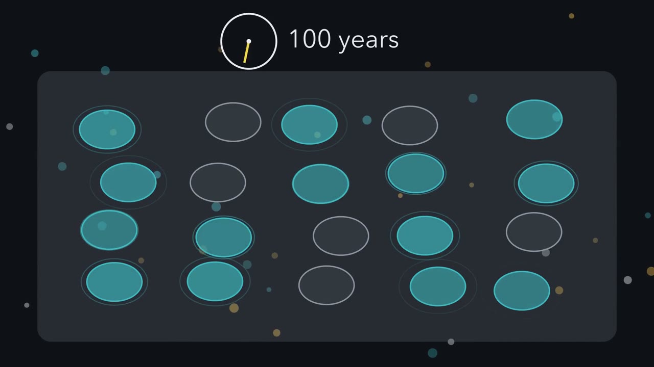 ▶ Watch A Region Outlasts Its Ponds · 3:17
Read the transcript of “A Region Outlasts Its Ponds”
Film transcript: A Region Outlasts Its Ponds
On this map, each pond's frogs last only about a decade. So why can the region still have frogs a century later? Each pond holds a local population, the frogs that live and breed there. The fields between are hostile ground. Ponds linked by dispersal like this form a metapopulation. Richard Levins asked the question simply. Forget how many frogs a pond holds. Each pond is either occupied or empty. Then follow one number: the fraction of ponds occupied.
Now let the map run. Ponds go grey as their populations die out. Others turn teal as colonists arrive. Which ponds are teal keeps changing, yet the teal fraction hovers near three quarters. Losses are the simple side of the ledger. Each occupied pond loses its population at a steady extinction rate. So total losses grow in a straight line with the fraction occupied. Gains are different.
Colonists must come from an occupied pond, and they can only found a population in an empty one. So gains need both kinds of pond. With no ponds occupied, there are no colonists. With every pond occupied, there is nowhere to land.
Between those two ends, gains rise and then fall in a hump. Where the gold hump meets the red line, gains equal losses. The occupied fraction settles there. That level is one minus the ratio of extinction to colonization, With these rates, it sits at three quarters. Now halve the colonization rate, and keep extinction the same. Does the occupied fraction halve too? Make your guess before the graph moves.
No. The hump shrinks, and the crossing slides only from three quarters to one half. What matters is the ratio of the two rates, not either one alone. Now push extinction up instead. The red line steepens, and the crossing slides left. When extinction equals colonization, the line only touches the hump at zero. No crossing above zero is left. So, in the model, a region keeps a species only while colonization beats extinction. No single pond has to last. Refounding balances loss at a level above zero. The model is deliberately simple. Its ponds are identical, all equally reachable, with rates that never change.
Real networks have big and small, near and far ponds. And a small network can lose every pond by chance, even when colonization wins.
From the film
- In the Levins model each patch is simply occupied or empty, and p is the fraction occupied.
- Occupancy rises by colonization, c p (1 − p), which needs both occupied and empty patches, and falls by local extinction, e p.
- Occupancy settles where gains balance losses, at p* = 1 − e/c, so a region keeps a species only while colonization beats extinction: c greater than e.
- Which patches are occupied keeps changing even when the fraction occupied does not.
- The model assumes many identical, equally reachable patches with constant rates; a small network can still lose every patch by chance.
The first film showed how a region outlasts its ponds. It left out three things: how fast a network is lost once the balance tips, what sets the two rates, and how to measure them on animals that hide. Visit a pond three times, hear no toads, and you still cannot say it is empty. Population growth asked whether one population grows (its growth factor per time step, lambda, above or below 1) and demography estimated its birth and survival rates; here the question moves up to a region of patches.
The one idea. A region can keep a species even though no patch keeps its population, as long as colonization beats extinction: the colonization rate c is greater than the extinction rate e. Then the fraction of patches occupied, p, settles at p* = 1 − e/c, the level where patches refounded balance patches lost.
Scope: this is the deterministic Levins model: many identical, equally reachable patches, constant rates, no attention to how many animals each patch holds. There p* is the long-run occupied fraction, not a fixed set of ponds. A real, finite network only wanders near p* for a while: once every patch is empty it stays empty, so a small network can eventually lose every patch by chance even when c is greater than e.
The ledger: colonization against extinction
For the first film’s metapopulation, local populations linked by dispersal across hostile ground, Richard Levins (1969) wrote the occupied-or-empty bookkeeping as a ledger:
In words The rate of change of occupancy is c times p times one minus p, minus e times p.
- dp/dt“d p d t”
- the rate at which the occupied fraction changesper year
- c“c”
- the colonization rateper year
- p“p”
- the fraction of patches occupied. Colonists come from these patches.
- 1 − p“one minus p”
- the fraction of patches empty. Colonists succeed only here.
- e“e”
- the local extinction rate: each occupied patch loses its population at this rate. Here e is a rate, not the number e ≈ 2.718.per year
Sanity check If p = 0 there are no colonists and no populations to lose, so nothing changes. If p = 1 there is no empty patch to colonize, so only the extinction term is left and occupancy can only fall.
Try one number
Take c = 0.4 and e = 0.1 per year, with half the patches occupied, p = 0.5.
Colonization: 0.4 × 0.5 × 0.5 = 0.1. Extinction: 0.1 × 0.5 = 0.05.
dp/dt = 0.1 − 0.05 = +0.05 per year, so occupancy is still rising.
Occupancy stops changing, at its equilibrium, when the two terms balance:
In words p star, the equilibrium occupancy, is one minus the ratio of extinction rate to colonization rate.
- p*“p star”
- the equilibrium fraction of patches occupied
- e“e”
- the local extinction rateper year
- c“c”
- the colonization rateper year
Sanity check With no extinction (e = 0), every patch ends up occupied, p* = 1; when e equals c, p* = 0.
Try one number
An invented middle case: c = 0.4 and e = 0.2 per year. e/c = 0.5, so p* = 1 − 0.5 = 0.5: half the patches occupied on average.
Where it comes from optional
1. Set dp/dt to zero: c p (1 − p) = e p.
2. Divide both sides by p (for any network that has occupied patches): c (1 − p) = e.
3. Divide by c and move p to one side: 1 − p = e/c, so p = 1 − e/c.
Need a refresher? rates and “per”
Predict. A network sits at p* = 0.75, with c = 0.4 and e = 0.1 per year. If e rises to 0.4, equal to c, the first film showed that no equilibrium above zero is left. Will the network be gone within two or three years?
Check your prediction
No. The ledger becomes dp/dt = −0.4 p², so occupancy falls at 0.4 × 0.75² = 0.225 per year at first, and the slide slows as fewer patches are left: about 0.47 is still occupied after 2 years, 0.39 after 3, and about one patch in five (0.19) after 10. Falling from 0.75 to 0.05 takes about 47 years here, against about 5.5 years if e were 0.8. Once e is at or above c, the closer e is to c, the slower the slide (working in Going deeper).
So a network at or just past its threshold can keep occupied patches for years: seeing animals does not show the region is persisting. The simulation runs these rules on 100 patches.
- Equilibrium p* = 1 − e/c
- 0.75
- Expected p at this year
- —
- Observed (this run)
- —
- Colonizations in the year: expected | observed
- —
- Extinctions in the year: expected | observed
- —
In this sketch: 100 identical patches, all equally reachable from every other, constant c and e, no rescue effect; the run starts with 75 patches occupied, and the random run is one draw (Resample for another). Rates apply in 0.05-year steps (a sketch choice); expected and observed counts differ by chance, since this is one random draw.
Keep the rule: occupancy settles at p* = 1 − e/c only when c is greater than e; patches keep changing state even when the fraction does not.
What sets the rates: dispersal, sources and rescue
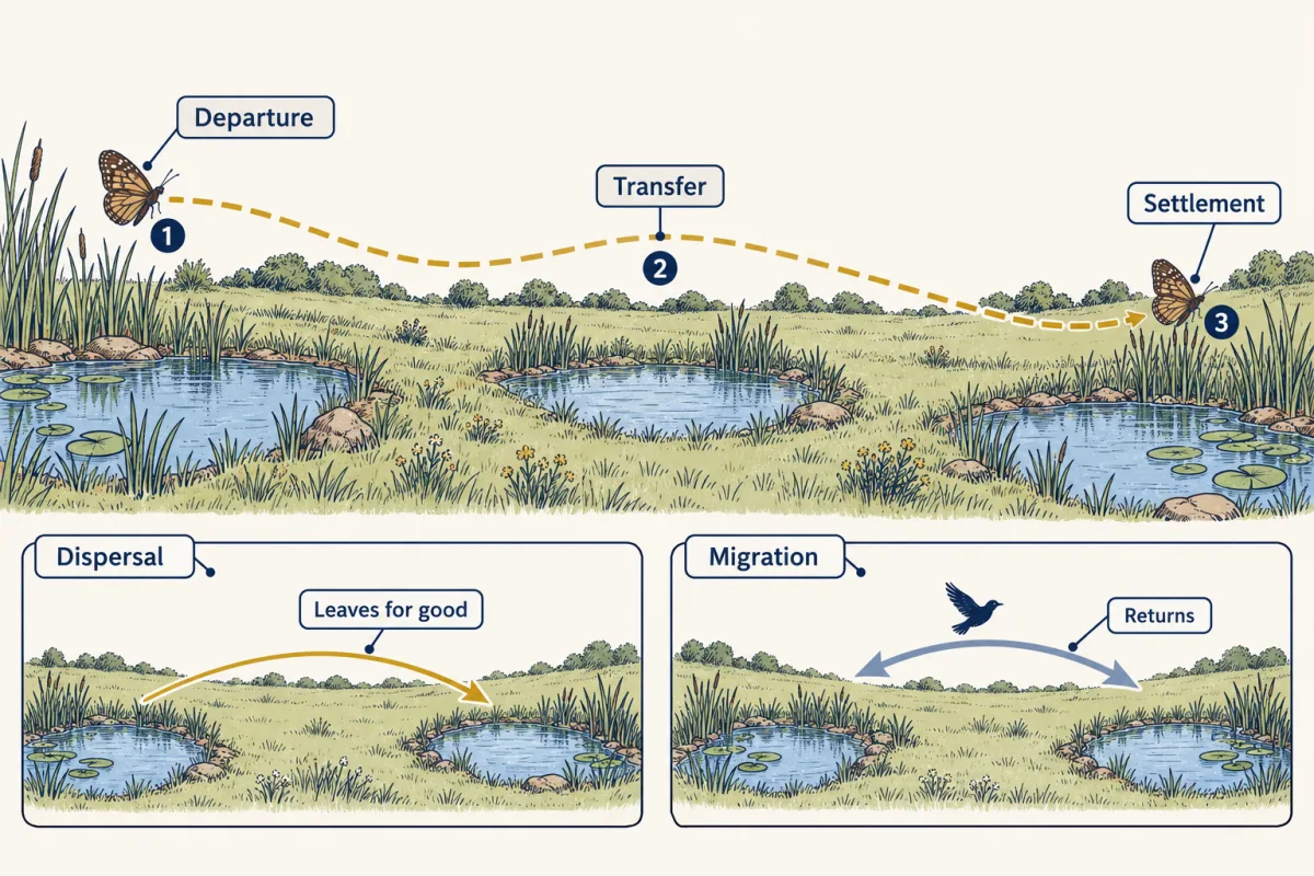
Dispersal is movement from where an individual was born, or last bred, to where it breeds next. It is what c is made of, in three stages that can be measured separately: departure, transfer across the landscape, and settlement. They need not share causes: in the Glanville fritillary butterfly in the Åland Islands of Finland, the factors that explained departure explained little of the variation in how far butterflies went (DiLeo and colleagues, 2022). Dispersal is not migration, a seasonal round trip: a migrating warbler returns to the same areas each year; a dispersing one changes where it breeds, and it may move again later. Dispersal also carries genes, the gene flow of drift, gene flow and competing explanations, with the arithmetic in population genetics.
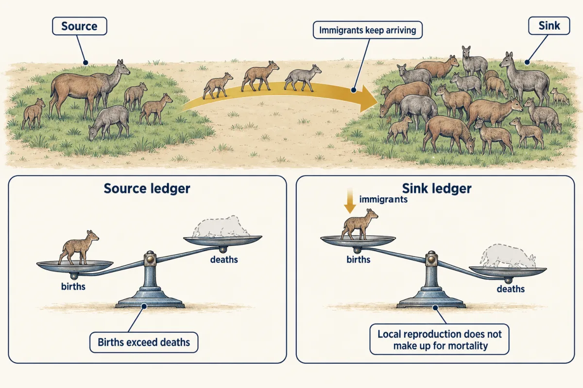
Levins treats every patch as equal. H. Ronald Pulliam (1988), in a different kind of model that follows births and deaths rather than occupied patches, let habitats differ. Each habitat keeps its own ledger: births and immigrants (arrivals) in, deaths and emigrants (departures) out. In a source, local births exceed local deaths, and the surplus emigrates. In a sink, local reproduction does not make up for local mortality, and the population persists only because immigrants keep arriving.
Predict. A meadow holds the most butterflies of any patch in the region, year after year. Is it a source?
Check your prediction
You cannot tell from the count. A sink fed by a strong source can be full of animals. Birth and death rates, and how many animals arrive and leave, label a source; abundance does not. That is also why a species can be found outside the conditions it can sustain, a point taken up in niches and distributions.
Two ways movement keeps patches occupied, often confused:
| What movement does | Where it enters the ledger | |
|---|---|---|
| Recolonization | refounds a patch after its population has gone | the colonization term, c p (1 − p) |
| Rescue effect (Brown and Kodric-Brown, 1977) | immigrants join a population that is still present and lower its chance of dying out | lowers e for patches that receive immigrants; the basic Levins model leaves it out |
Linking patches with corridors, strips of habitat between them, can raise c; where immigrants rescue populations that are still present, it can also lower e. But a corridor adds habitat area as well as connection, so an experiment must pull the two apart (design problem below). Connectivity does not help in every model (Going deeper).
A sink, a rescued population, a corridor that raises c: each claim rests on knowing which patches are occupied, year by year, and that starts with whether the species was there at all.
Read the transcript of “Two Kinds of Zero”
Film transcript: Two Kinds of Zero
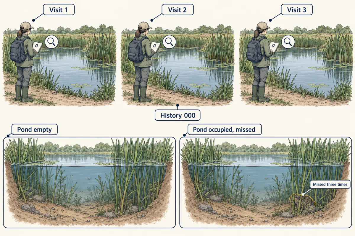
Sources, rescue and corridors all rest on one record: which ponds are occupied. Three visits, no toads heard. Is the pond empty? A survey sheet would simply score it as a zero. A zero on a survey sheet has two meanings. The pond may truly be empty. Or toads were there, and the observer missed them on every visit. So surveyors return to each site several times in one season, while occupancy is assumed not to change. Each visit scores a one for detected, and a zero for not. Three visits give a history, like 110, or 010. A 010 history shows a pond that was occupied, and missed twice. Take eight ponds that really hold toads. Each visit detects them with a probability of one half, independently of the other visits. After three visits, how many ponds look empty?
About one, on average. With independent visits, three misses in a row happen one time in eight. Each extra visit halves that chance again. Harder species are missed more often. When each visit finds them only 3 times in 10, about 1 occupied pond in 3 comes out all zeros. No single site can settle it, but many sites together can.
Across them, the pattern of histories carries the answer. A model estimates the chance of detection and the fraction occupied, together. A naive count lights only the ponds with a detection. The corrected estimate is higher, because some silent ponds hold toads. Treat every silent pond as empty, and occupancy is counted low. Darryl MacKenzie and colleagues published this method. They tested it on volunteer surveys of wetlands in Maryland, made two years earlier. American toads were detected at least once at only about a third of the wetlands analysed. The model put the fraction occupied near one half. The method has rules of its own. Occupancy must stay fixed across a season's visits.
Toads must never be recorded where they are absent. And detection must be independent among sites and among visits. So a zero is a result of looking, not proof of absence. How hard you looked belongs in the analysis, before any pond is called empty.
From the film
- A survey zero can mean the species is absent, or that it was there and missed.
- A history such as 010 shows a site that was occupied and missed on two of three visits.
- If each visit independently detects an occupied site with probability 0.5, three visits all miss it one time in eight.
- Visiting each site several times, while occupancy stays fixed, lets a model estimate detection and occupancy separately.
- In Maryland in 2000, American toads were detected at 10 of 29 wetlands analysed, about 0.34, but estimated to occupy 0.49.
Two kinds of zero: occupancy
The second film’s repeat visits estimate occupancy within one season: the same kind of quantity as p in the Levins model, now measured in the field. It left out time. Across years, colonization and extinction are read from which sites switch between occupied and empty, and there the same zeros do more damage.
Predict. A survey team scores every 000 history (no detection on any of three visits) as an absence, year after year. Will the network look more or less occupied, and more or less changeable, than it is?
Check your prediction
Less occupied and more changeable. A missed population is scored as a local extinction, and finding it again as a colonization, so both transitions look more frequent while occupancy looks lower than it is. An illustration in yearly probabilities: empty ponds are colonized with probability 0.3 and occupied ones lost with probability 0.1, keeping three ponds in four occupied. If detection is 0.3 on each of three visits a year, independently, an occupied pond is missed on all three with probability 0.7³ = 0.343. Apparent extinction is the true 0.1 plus surviving populations missed, 0.9 × 0.343: about 0.41, four times the truth. Apparent colonization comes out near 0.40, and only 0.75 × (1 − 0.343), about 0.49, of ponds show a detection. This is error in the record, not a measure of how near the network is to collapse. Dynamic occupancy models, which estimate detection alongside colonization and extinction, correct for this; their yearly probabilities are field counterparts of c and e, not the same numbers (Going deeper).
Counting animals: mark-recapture
Occupancy surveys repeated across years show how often sites are colonized and lost; source-sink claims need births, deaths and movement, which need data on individuals. The simplest count of hidden animals is a proportion: the marked share of a second catch should match the marked share of the whole population.
In words N, the population size, is the first catch times the second catch, divided by the marked animals in the second catch.
- N“N”
- the estimated number of animals in the populationanimals
- n1“n one”
- animals caught, marked and released on the first occasionanimals
- n2“n two”
- animals caught on the second occasionanimals
- m2“m two”
- animals in the second catch that already carry a markanimals
Sanity check If every animal in the second catch is marked (m2 = n2), N = n1: you had already marked everyone. The fewer marked animals you recatch, the larger the estimate. If you recatch none, m2 = 0 and the formula breaks down.
Try one number
Round invented numbers: mark 10, later catch 10, and 2 of them are marked.
N = 10 × 10 / 2 = 50. Check: 2 of 10 is one fifth, and 10 marked animals are one fifth of 50.
Where it comes from optional
Set the two marked fractions equal: m2 / n2 = n1 / N. Multiply both sides by N and by n2: m2 × N = n1 × n2. Divide by m2: N = n1 × n2 / m2.
Need a refresher? rates and “per”
Worked problem (invented data). You catch and mark 50 animals on the first occasion (n1 = 50), release them, and later catch 90 (n2 = 90), of which 20 are marked (m2 = 20). Assume the population is closed (no births, deaths or movement between occasions), every animal is equally catchable, and marks are neither lost nor misread.
- Lincoln-Petersen. The marked fraction 20/90 estimates 50/N, so N = n1 x n2 / m2 = 50 x 90 / 20 = 4,500 / 20 = 225 animals.
- Chapman. The plain estimator runs high when samples are small; Chapman’s version adds one to each count, which reduces that bias and avoids dividing by zero if no marked animals are recaught:
N = (n1 + 1)(n2 + 1) / (m2 + 1) - 1
Add one to each count: 50 + 1 = 51, 90 + 1 = 91 and 20 + 1 = 21. Then N = (51 x 91) / 21 - 1 = 4,641 / 21 - 1 = 221 - 1 = 220 animals.
The overlap is 20, not 90. And 220 is an estimate resting on every assumption, not a head count.
Predict. Suppose marked animals learn to avoid traps, so they are less likely than unmarked ones to be caught the second time. Will the estimate come out too high or too low?
Check your prediction
Too high: trap-shy marked animals are under-represented in the second catch, so m2 is too small and N too large. Trap-happy animals do the reverse, inflating m2 and shrinking N. Photo identification, as in a 2018 survey of free-roaming dogs in Quito, Ecuador, avoids handling but can mismatch individuals.
Movement also breaks closure. Traditional live-encounter mark-recapture estimates apparent survival, the chance an animal is alive and still in the study area: one that emigrated permanently looks exactly like one that died, so the dispersal that keeps a metapopulation going blurs the death rates a source-sink claim needs.
Design problem
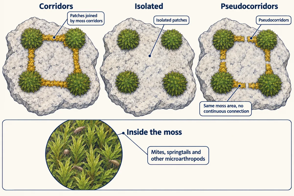
Gonzalez and colleagues (1998) worked with moss on limestone rocks in Derbyshire, England, home to tiny mites, springtails and other microarthropods. They cut the moss into patch systems of three kinds: patches joined by moss corridors; isolated patches; and patches with pseudocorridors, corridors of similar moss area broken by a small strip of bare rock, so with no continuous connection. After six months, species losses were 14.5% in connected landscapes and 41% in the isolated and pseudocorridor treatments. What can you conclude, what can you not, and how would you improve the study?
Saved in this browser only.
One way to do it
What the pseudocorridor buys. It adds similar moss area without the connection, and it lost species like the isolated patches, so the difference points to connection rather than added area.
What it is consistent with. Fewer losses where patches connect fits a rescue effect, immigrants arriving through corridors propping up dwindling populations. But no movement was tracked, so recolonization after loss, or different conditions in connected moss, are not ruled out.
Improvements.
- Mark animals, or use genetic assignment, to measure movement through corridors.
- Record each species in each patch at several times, to separate fewer extinctions from more recolonizations.
- Run it longer than six months, and replicate across rocks and seasons.
- Keep the scale. This is moss on rocks, centimetres to metres, with animals of short generation time. It says nothing directly about forests or mammals.
A larger, longer contrast. Damschen and colleagues (2019) censused 239 plant species yearly for 18 years in connected and unconnected longleaf pine savanna fragments in South Carolina, estimating colonization and extinction separately, which the moss study could not: colonization 5% higher and extinction 2% lower each year in connected fragments, and nearly 14% more species after almost two decades. It too stays in its system: one site, plants, one corridor geometry.
Going deeper
Dispersal stages and migration
DiLeo and colleagues (2022) reconstructed Glanville fritillary dispersal by genetic assignment across five years and 232 habitat patches, and also found no effect of distance on survival after settling. Migration varies too: in some insects, such as painted lady butterflies, the cycle is completed over several generations.
Small networks can be lost by chance
In an illustrative simulation with c = 0.15 and e = 0.1 per year (p* = 0.33), started half occupied, most 10-patch networks lost every patch within 100 years, while 100-patch networks kept the species. In a small network, c greater than e is necessary but not sufficient.
The exact path when c equals e
With c = e = 0.4 from a start of 0.75, dp/dt = −0.4 p² has the solution 1/p = 1/0.75 + 0.4t. After 10 years 1/p = 1.333 + 4 = 5.333, so p is about 0.19; reaching p = 0.05 (1/p = 20) takes (20 − 1.333)/0.4, about 47 years. With e = 0.8 the ledger is dp/dt = −0.4 p (1 + p), and solving it the same way gives about 5.5 years.
Rescue makes e depend on p
In the Levins model the extinction rate does not depend on regional occupancy. Adding rescue makes e fall as p rises and, in some versions, can produce alternative stable states.
When connectivity hurts
In simulations of 21 competing bird-like species, Schippers and colleagues (2015) found that greater connectivity sped up diversity loss. That is a model result, a caution about extrapolation, not a field finding.
Spatial structure and predator-prey cycles
C. B. Huffaker (1958) kept a predatory mite with its prey mite on arrays of oranges. With the food spread out and movement partly blocked, the most complex arrangement sustained three successive oscillations before the run ended: a finite run in one preparation, not proof of permanent coexistence, but a case that spatial structure can prolong a predator-prey interaction. Predator-prey cycles return in predation.
Dynamic occupancy and the symbol ψ
Survey papers write occupancy as ψ (psi); this lesson keeps p, to match the Levins model. Later work by MacKenzie’s group extended the method across seasons, estimating colonization and local extinction without mistaking missed detections for losses. Those yearly probabilities, written γ and ε, are not the Levins c and e: Levins refounds an empty patch at rate c p, which grows with occupancy, and his c and e are continuous rates. Linking the two takes an explicit model of how colonists spread.
Your notes
Select any text in the lesson to highlight it or add a note to it. Your highlights and notes are saved in this browser and collected in your notebook.
This browser is not letting the site save anything (a private window or strict privacy settings), so highlights and notes will be lost when you leave the page.
How we measure it
Mark-recapture
Animals are caught, marked or photographed so that each can be recognised, and released; a later sample records how many are already marked. Under closure, equal catchability and correct matching, the marked fraction of the second sample estimates the marked fraction of the whole population.
Repeat-visit occupancy surveys
Each site is visited several times within a period when its occupancy is assumed not to change, and detection or non-detection is recorded each time. The detection histories let a model estimate the probability of detection and the fraction of sites occupied separately, provided the species is never recorded where it is absent and detection is independent among sites and among visits, with any variation in it modelled.
Corridor experiments with area controls
Habitat fragments are connected or left isolated, and some fragments receive about the same added habitat area in a form that does not connect them. Comparing the treatments separates the effect of connection from the effect of extra area.
Genetic assignment of dispersers
Individuals are genotyped and assigned, with some uncertainty, to the patch they most likely came from, so that departure, straight-line dispersal distance and settlement can be estimated for successful dispersers without following each animal.
Practice questions on this lesson (3) → MCAT-style, original, each with an explanation
Where this lesson fits
Before thisReview first
- Population Growth and RegulationThis course · Lesson 14
You need growth factor lambda and constant per-capita rates from there before treating colonization and extinction as rates.
- Demography and SurvivorshipThis course · Lesson 13
Birth and survival rates from there are what the source and sink ledger of births and deaths uses.
- Distributions, Niches and TolerancesThis course · Lesson 12
You need to know why a species occupies some places and not others before asking which patches are occupied.
After thisStudy next
- Predation and Community EffectsThis course · Lesson 17
Spatial structure can prolong predator-prey cycles, which this lesson first showed with Huffaker's oranges.
- Island BiogeographyThis course · Lesson 20
Colonization balancing extinction sets species number on islands, the same ledger applied to species instead of patches.
- Conservation and RestorationThis course · Lesson 25
Corridors, rescue and small networks lost by chance are used there to judge how to protect fragmented populations.
Elsewhere on the siteFilms, simulations and method films in other courses
- Grow a population, then add limitsSimulation · Biology
Shows how a single population levels off, a contrast to a region's occupied fraction settling at balance.
Suggested by an AI model from the lessons themselves, then checked. How we use AI
Finish line
Test yourself
8 questions
Practice and MCAT-style, with explained answers.
Next · Lesson 16
Competition
One competitor grows twice as fast as the other. Why does it not always win?
Continue →