Ecology and Evolution · Unit 6: Global change and decisions
New to this? Review it at high school level: The Chesapeake Under Pressure
Conservation and Restoration
Rewritten on : new text, flashcards and film. Your notes and highlights stay, but the text around them may have moved.
In 1995, eight female pumas from Texas were released into the Florida panther population. What did that change, and how would you know?
Pause when the reading reaches a film, and offer to play it. Saved on this device.
Watch the film now, or keep listening
Builds on:Population Growth and RegulationDrift, Gene Flow and Competing ExplanationsMovement and Spatial PopulationsWhy these?
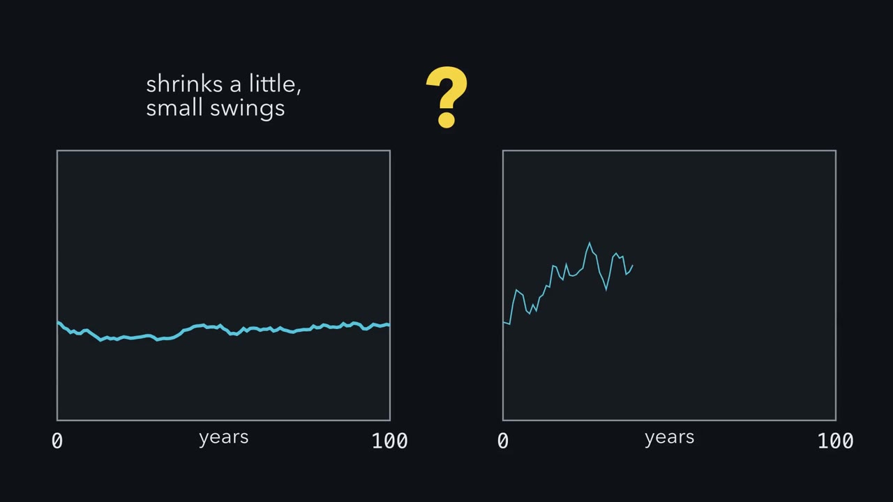 ▶ Watch Trend and Chance · 3:23
Read the transcript of “Trend and Chance”
Film transcript: Trend and Chance
Which population is in more danger? One shrinks a little on average each year. The other grows a little, but its numbers swing wildly. Both start with fifty animals. Put one population on a chart. Each blue line is one possible run of its numbers. The red dashed line is the floor, a number too low to recover from. Two things move the line. The gold arrow is the trend, the average yearly change on a log scale.
Around it the line jitters up and down. Those are the swings, the good years and bad. Now run the same population two hundred times. The runs fan out. Some touch the floor. The fraction that touches it is the risk. That is the idea behind a population viability analysis A real one runs a fuller model many times, and counts the runs that fall. Turn two dials, one at a time. Widen the swings, and more runs touch the floor. Raise the start, and fewer runs do. Now tilt the gold arrow down, so the population shrinks on average. Will starting with ten times as many animals save it?
Over one century, the bigger start helps a lot. Far fewer runs touch the floor. But keep the clock running. Over a thousand years, nearly every run reaches it. The bigger population bought time, not safety. With the arrow pointing down, every start reaches the floor in the end. How soon depends on the trend, the start and the swings together. Tilt it up to plus point oh two, and most runs stay clear. With few animals, one unlucky litter can decide the outcome. So chance in single births and deaths weighs most near the floor.
Genes can tilt the arrow too. Fewer animals means more mating among relatives. Inbreeding can lower survival and fertility, so the trend tilts down and numbers fall further. This loop is called the extinction vortex. Back to the two populations. The shrinking one will reach the floor in time, however big it starts. The growing one can escape. Its risk still depends on trend, size and swings together. This gives managers a target, for one population in one habitat. A minimum viable population is the smallest start that keeps the risk below a chosen level, over a chosen time. So conservation starts by removing the cause of decline. Alongside it, numbers, connections and genes can lift the trend or cut the risk.
But in this model, without a trend above zero, size only buys time.
From the film
- In a simple model of one population, if the trend, its average yearly change on a log scale, is zero or below, the population reaches the floor in the long run; how soon depends on the trend, the size and the swings together.
- In this model, without a trend above zero, a bigger population only buys time: over a long enough span nearly every run reaches the floor.
- Chance in which animals survive and breed matters most when numbers are small, and inbreeding can pull the trend down further.
- A population viability analysis runs a fuller model of the population many times and reports the fraction that falls to the floor within a chosen time.
- So conservation starts by removing the cause of decline; alongside it, numbers, connections and genes can lift the trend or cut the risk.
In 1995, managers released eight female pumas from Texas into southern Florida, where a small, inbred population of Florida panthers still lived. By 2010 panther numbers had about tripled, and heterozygosity, a measure of genetic variation, had doubled.
Was that a success, and how would you know? The first film’s rule is the yardstick.
The one idea. A population’s trend is its average yearly change in numbers on a log scale. If the trend is zero or below, the population reaches the floor (zero, or a number too low to recover from) in the long run, and size only buys time; a trend above zero makes lasting possible, though not certain. How soon, and how likely within a given time, depends on the trend, the size and the swings (the ups and downs from year to year) together. So conservation starts by removing the cause of decline. Alongside it, numbers, connections and genes can lift the trend or cut the risk.
Scope, stated once: this holds in a simple model of one population whose log numbers wander with a steady trend and steady swings, with no immigration and no return from the floor. Real analyses add crowding, Allee effects, catastrophes and immigration, so the rule sorts causes; it is not a law.
Graeme Caughley argued in 1994 that most populations are small because something, such as habitat loss or overharvest, drove them down, so finding and removing that cause usually comes first. The risks of small numbers may still need managing at the same time.
Why small populations are fragile
Mark Shaffer (BioScience, 1981) sorted the chance events that threaten small populations into four kinds. They interact, and several act on both the trend and the swings.
Demographic stochasticity is chance in individual fates: which animals happen to survive, and how many offspring, of which sex, each produces. Suppose a population’s last breeding female has five young. The chance that all five are male is (1/2)5 = 1/32, about 3%. In a population of thousands such runs of luck average out.
Environmental stochasticity is variation from year to year in weather, food and the populations of competitors, predators and disease that a population depends on.
Predict. A drought year hits a population of 10 and a population of 10,000. Does the larger one escape the drought the way it escapes an unlucky run of all-male litters?
Check your prediction
No. A drought hits every individual at once, so it does not average out with size the way demographic chance does. Size gives a bigger cushion, not a smaller shock.
Catastrophes, such as fires, hurricanes and epidemics, are the extreme swings. The fourth kind is genetic. In a small population genetic drift (chance change in allele frequencies) erodes variation, the raw material for adaptation, and mating among relatives raises inbreeding, which exposes harmful recessive alleles and feeds the first film’s vortex. Drift’s arithmetic belongs to population genetics (rate of loss in Going deeper).
Michael Gilpin and Michael Soulé named the first film’s loop an extinction vortex in 1986. Some species also show an Allee effect: at low density, individuals find mates or defend against predators less well, so the trend itself falls just when numbers are lowest. The rates that drive these models come from life tables and population growth.
MVP and PVA: risk as a probability
How many individuals are enough? Shaffer’s answer: none, until you choose a standard. He defined a minimum viable population (MVP) as the smallest isolated population, in a given habitat, with a chosen probability of persisting for a chosen time. As a tentative example he suggested a 99% chance of persisting for 1,000 years. Change the probability, the horizon or the habitat, and the MVP changes.
A population viability analysis (PVA) estimates that probability as the film did, by running a model many times, but with a real species’ complications: survival and birth rates by age or stage, their variation between years, density dependence (rates that change with crowding), catastrophes and, sometimes, inbreeding. Like a forecaster’s “30% chance of rain”, it reports the fraction of runs that go extinct, or fall below a chosen threshold, within the horizon.
Are such forecasts right? In 2000, Barry Brook and colleagues fitted PVA models to the first half of each of 21 long-term ecological data sets and predicted the second half. Predicted risks of decline matched observed outcomes closely, with no significant bias. That supports PVA within populations and spans like those tested, not any single forecast. PVA is most often recommended for comparing management options rather than for its absolute numbers, and even rankings need checking (Going deeper).
Worked problem, part A. For one hypothetical species in one habitat (invented numbers), a PVA is run 1,000 times from each of three starting sizes, over 100 years. Extinction means zero individuals by year 100. Assume the model’s vital rates (survival and birth rates) and their variation are correct and the habitat stays as it is.
| Starting size N0 | Runs extinct | Extinction probability |
|---|---|---|
| 20 | 120 | 120 / 1,000 = 12.0% |
| 50 | 37 | 37 / 1,000 = 3.7% |
| 100 | 8 | 8 / 1,000 = 0.8% |
Probabilities are extinct runs divided by total runs. Suppose managers choose at most 5% extinction risk in 100 years. N0 = 20 fails. N0 = 50 passes, with persistence 1 - 0.037 = 96.3%. So 50 is the smallest tested size that meets the target. Sizes between 20 and 50 were never run, so the true threshold could lie anywhere in that range.
Predict. 3.7% is below the 5% target, but only 1,000 runs stand behind it. Would you sign off on 50 animals?
Check your prediction
Only narrowly: 1,000 runs are too few to be sure. A fraction counted from runs has sampling error, the Monte Carlo error. Its standard error is the square root of (0.037 x 0.963 / 1,000), about 0.006, so a rough 95% range (two standard errors either side) is 2.5% to 4.9%. The upper end sits just under 5%, so more runs would be needed to be confident.
Problem A held the vital rates fixed. If inbreeding keeps accumulating, survival or fertility can fall, lowering the trend; a PVA must model that or say it leaves it out. The second film follows a well-known genetic rescue: adding animals from another population to lift fitness that inbreeding has lowered.
Read the transcript of “Eight Females from Texas”
Film transcript: Eight Females from Texas
A model that holds survival fixed can miss something. If inbreeding keeps building, survival or fertility can fall, and the trend tilts down. Can adding new genes tilt it back up? Southern Florida held a small, isolated population of Florida panthers. Its animals showed signs linked to inbreeding: kinked tails, heart defects and poor sperm. Put them on the first film's chart.
Numbers sit close to the floor. Inbreeding can lower survival, so the gold arrow tilts down. The vortex is turning. In 1995, managers tried a genetic rescue. They released eight female pumas from Texas into the Florida population.
Texas pumas belong to the same species, from a separate population. Adding animals to a population that still exists is called reinforcement. The aim was genetic: to reverse inbreeding by bringing in new gene versions. Over the following years, more and more panthers carried both Florida and Texas ancestry. Biologists call such animals admixed. To judge the rescue, track two things. One is the head count. The other is heterozygosity: the share of gene positions where an animal carries two different versions. In 2010, a team led by Warren Johnson reported the result.
Numbers had about tripled. Heterozygosity had doubled. Survival and fitness measures had improved. On the chart, the arrow tilts up. The same report warned that habitat loss and persistent inbreeding remained concerns. So, if habitat keeps shrinking, will the climb continue?
In 2024, a team led by Dave Onorato returned, with records from 1,192 panthers. The genetic benefits had lasted through five generations. Yet the population stabilised, and then declined, during 2016 to 2020. The genetic benefits held, yet the climb stopped. A population gain from genetic rescue may not last if other causes of decline remain. How did the teams judge the rescue? They compared admixed with non-admixed animals, and the years after the release with the years before. Both comparisons came from a single population. So genetic rescue can ease inbreeding and lift survival and births. But it does not by itself remove other causes, such as habitat loss or road deaths.
Address those too, or the gain may fade. Genes and habitat work together.
From the film
- In 1995 eight female pumas from Texas were released into the small, inbred Florida panther population, a planned genetic rescue.
- By 2010 panther numbers had about tripled and heterozygosity, a measure of genetic variation, had doubled.
- A 2024 follow-up found the genetic benefits lasting through five generations, while the population stabilised and declined during 2016 to 2020.
- Genetic rescue can ease inbreeding and lift the trend, but it does not by itself remove other causes of decline, such as habitat loss, so a population gain from it may not last.
Census size and effective size
The second film left open how far a head count overstates genetic size, how firm the causal reading is, and whether one cat is typical.
The census size N is the number of individuals you count. The effective size Ne is the size of an idealised population, with equal sexes, random mating and family sizes that vary only by chance, that would lose genetic variation at the same rate. Ne is usually smaller than N, because uneven sex ratios, unequal numbers of offspring and swings in population size all speed drift: if a few males father most young, fewer parents pass on genes than the count suggests. For an unequal sex ratio alone, with Nm breeding males and Nf breeding females:
Ne = 4 Nm Nf / (Nm + Nf)
Worked problem, part B. Suppose 50 adults breed: 10 males and 40 females. Assume discrete generations and that sex ratio is the only departure from the ideal.
Predict. Fifty animals breed. Is the population’s effective size 50?
Check your prediction
No. Ne = 4 x 10 x 40 / (10 + 40) = 1,600 / 50 = 32, so Ne/N = 32 / 50 = 0.64.
Convert a genetic guideline. Frankham, Bradshaw and Brook (2014) recommended Ne of at least 100 to keep the loss of total fitness to 10% or less over five generations, and at least 1,000 for long-term evolutionary potential. At Ne/N = 0.64, Ne = 100 needs about 156 adults (rounded up to whole animals in Going deeper).
- Census of breeders N
- 50
- Ne = 4 NmNf / (Nm + Nf)
- 32
- Ne / N
- 0.64
- Adults needed for target (exact)
- 156.25
- Smallest whole-animal group at this ratio that reaches the target
- 32 males + 128 females = 160 adults, Ne = 102.4
In this sketch: only the sex ratio lowers Ne; discrete generations, and other causes of low Ne are ignored; the sex ratio is held constant as the population grows.
The guideline is an effective size, not a head count: convert it with the Ne/N of the population in question. Equal numbers of each sex give Ne = N, and any imbalance gives less.
This assumes the ratio holds and ignores the other causes of low Ne, which in wild populations often push Ne/N much lower. Frankham’s 100/1,000, like the older 50/500 rule, is about effective size: neither is a census target.
How firm is the panther reading?
Both of the second film’s comparisons come from one population with no replicated control, and habitat, prey and road deaths changed alongside ancestry. The associations between admixture and fitness are strong, but how much to credit to genes rather than habitat or road deaths remains inference.
Is one cat typical?
Genetic rescue does not rest on the panther alone: a 2015 meta-analysis found that outcrossing inbred populations improved fitness in 92.9% of 156 cases judged to carry a low risk of outbreeding depression (reduced fitness after crosses between genetically different populations, sometimes appearing only in the grandchildren of the cross).
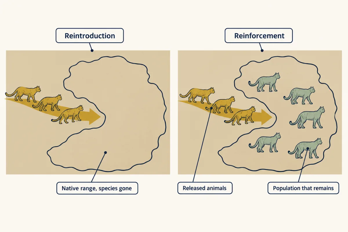
IUCN guidance asks for strong evidence that the threats that caused any earlier loss have been identified and removed or sufficiently reduced first, as Caughley argued.
Habitat tools: changing the trend and the swings
Removing the cause of decline often means protecting or restoring habitat, though for some populations it means curbing harvest, invasive species, disease or pollution; diagnose the driver first. Protection and restoration aim to raise survival, births and the number of animals the land can hold; corridors allow immigration, recolonisation and gene flow. Each can lift the trend or cut the risk, depending on species and landscape.
Protected areas. Across terrestrial sites worldwide, Gray and colleagues (2016) found sample richness (species recorded per sample) 10.6% higher and abundance 14.5% higher inside protected areas than outside. Most of that advantage was explained by land-use differences between the sites, and rarefied richness (species counts adjusted for sample size) and endemism (a measure weighted toward species with small ranges) did not differ significantly. The comparison is observational, since reserves are not placed at random; matching protected sites with similar unprotected ones gives a cleaner estimate. In Costa Rica, Andam and colleagues (2008) found that about 10% of protected forest would otherwise have been cleared, and that simpler comparisons overstated that benefit by more than 65%.
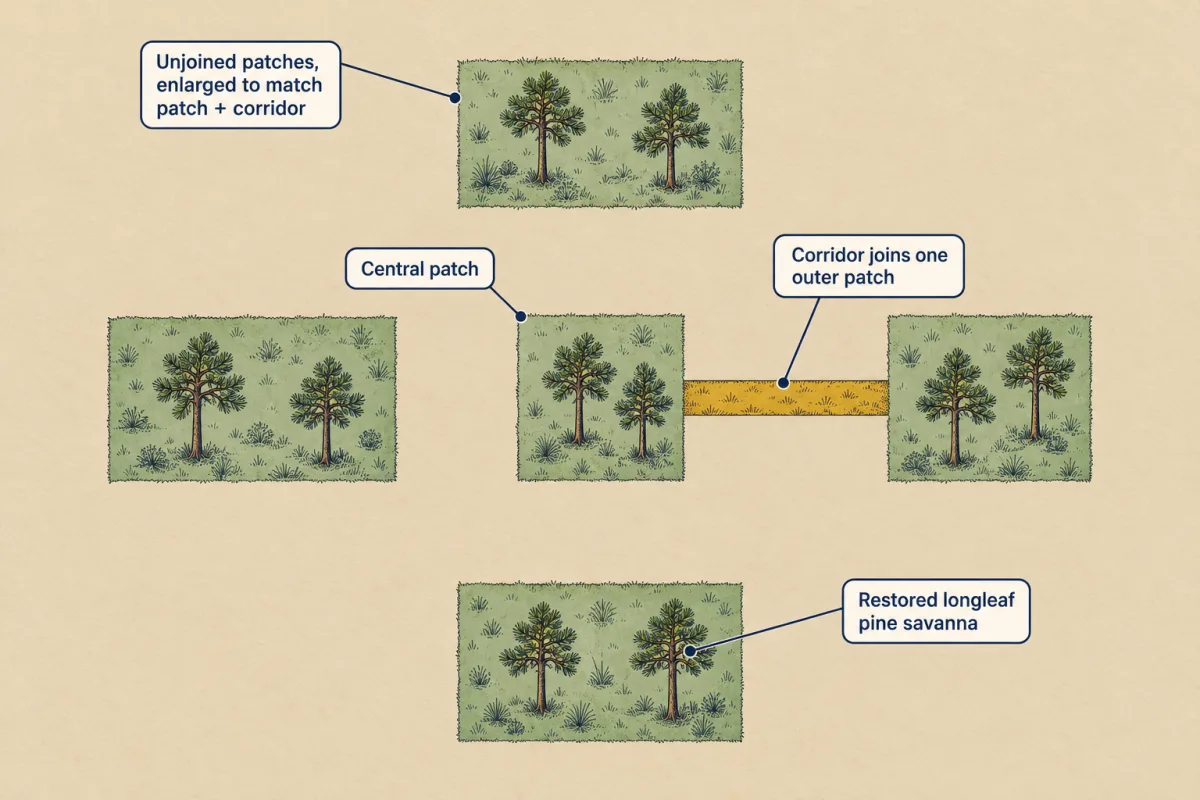
Corridors. At the Savannah River Site in South Carolina, in restored longleaf pine savanna, Damschen and colleagues followed plant species for 18 years in patches of equal area, some joined by corridors. Connected patches gained species faster, lost them more slowly and ended with more species. The study was replicated in ten experimental landscapes, but at one site in one ecosystem, so it does not establish how corridors work everywhere. The prediction comes from island biogeography and spatial populations.
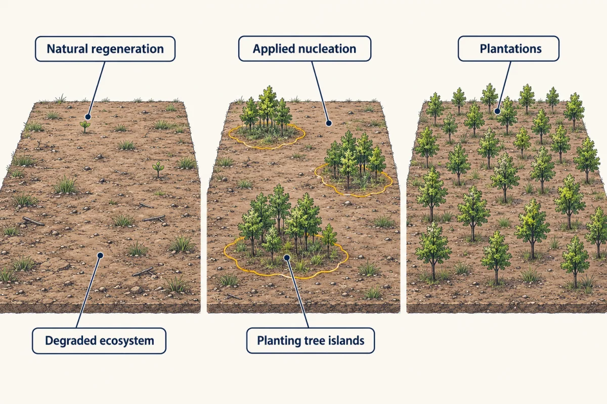
Restoration. The Society for Ecological Restoration defines it as assisting the recovery of a degraded, damaged or destroyed ecosystem. In southern Costa Rica, Karen Holl and colleagues compared natural regeneration, applied nucleation (planting tree islands) and plantations at 13 sites. After about a decade, planting raised recruitment (new young trees establishing) of animal-dispersed trees, yet tree-recruit composition in every treatment remained distinct from reference forest (intact forest used for comparison).
Predict. Across hundreds of recovery studies, does actively restoring a site bring its ecosystem back faster than simply ending the disturbance?
Check your prediction
Not on average. A 2018 global analysis of 400 recovery studies found that ecosystems rarely recovered completely within the study periods, and that active restoration did not, on average, give faster or more complete recovery than simply ending the disturbance, though few studies compared the two directly.
Action in general still beats doing nothing: a 2024 meta-analysis of 665 trials with no-action comparisons found that it improved biodiversity or slowed its decline in about two-thirds of cases.
Decisions with competing goals
Evidence says what an option is likely to do, not which outcome matters most. For endangered sockeye salmon of Cultus Lake in British Columbia, Gregory and Long (2009) described a structured decision process that set out biological, social and economic objectives, the alternatives and their predicted consequences, so that the fishery agencies, First Nations and commercial fishers involved could see the tradeoffs explicitly. Climate change shifts all of these options (global change), and the final lesson, the evidence workshop, practises weighing such studies together.
Design problem
A small, isolated mammal population shows signs of inbreeding (heart defects, low sperm quality, poor survival of young), and its habitat is still shrinking. Managers propose bringing in animals from another population of the species. Starting from the panther teams’ two comparisons, what would you add so the result says more than one population can?
Saved in this browser only.
One way to do it
Keep the panther design (a baseline of counts, survival, recruitment, heterozygosity and defect rates, then ancestry for every animal you can type), and record habitat loss, prey and road deaths alongside ancestry, to weigh their effects. If several isolated populations need help, release into some sooner than others, so the later ones serve as a comparison. State whatever limit remains.
Weigh outbreeding depression and disease carried by the newcomers. If the habitat keeps shrinking, a genetic gain may be temporary.
Going deeper
The exact interval and the IUCN criterion
In Problem A, a more exact interval method puts the upper end at about 5.1%. For comparison, the IUCN Red List can classify a taxon as Endangered under its criterion E when a quantitative analysis gives at least a 20% probability of extinction within 20 years or five generations, whichever is longer, up to 100 years.
Checking PVA rankings
In a 2017 test, rankings held across model structures for the dominant threats but not for smaller effects, and a 2020 appraisal rated fewer than one in five of 160 published PVAs as high quality.
The rule as a formula
The trend averages change in log numbers, so it never exceeds the average proportional change and can sit well below it when swings are large: a year that halves numbers and one that adds half average no proportional change, but a log trend of about -0.14.
For log numbers moving as a smooth random walk (a diffusion) with steady trend and swings and an absorbing floor, the chance of ever reaching the floor is 1 if the trend is zero or below. Above zero, a standard formula gives it in the smooth model. For yearly steps, as in the films, it is only an approximation, to be checked by simulation.
In words Floor over start, raised to the power two times the trend over the variance of the swings.
- floor“floor”
- the number too low to recover fromanimals
- start“start”
- the starting numberanimals
- trend“trend”
- average yearly change in log numbers, above zeroper year
- variance“variance”
- variance of the yearly swings in log numbersper year
Sanity check As the trend falls toward zero, the power shrinks toward 0 and the chance rises toward 1, matching the rule that a trend of zero or below makes reaching the floor certain.
Try one number
Need a refresher? powers and roots · rates and “per”
Drift and the loss of variation
In the ideal model, expected heterozygosity falls each generation by 1/(2Ne) of what remains. In Problem B, at Ne = 32, that is about 1.6% per generation, roughly 15% over 10 generations.
Effective size and the genetic guidelines in numbers
At Ne/N = 0.64, Ne = 100 needs 100 / 0.64 = 156.25 adults. With whole animals at one male to four females, 32 males and 128 females (160 adults) give Ne = 4 x 32 x 128 / 160 = 102.4, which clears 100. Frankham and colleagues give meta-analytic averages of Ne/N of about 0.1 to 0.2, which would put Ne = 100 at roughly 500 to 1,000 adults. A standardised median minimum viable population (MVP) of 4,169 individuals across 212 species (Traill and colleagues, 2007) summarises a literature and is not a target for any species.
The corridor experiment in numbers
At the Savannah River Site, Damschen and colleagues followed 239 plant species for 18 years. Annual colonization rates were 5% higher and local extinction rates 2% lower in connected patches, and connected patches ended with about 200 species against 176. Unconnected outer patches were of two kinds: rectangular, or with dead-end side strips (“wings”).
Your notes
Select any text in the lesson to highlight it or add a note to it. Your highlights and notes are saved in this browser and collected in your notebook.
This browser is not letting the site save anything (a private window or strict privacy settings), so highlights and notes will be lost when you leave the page.
How we measure it
Population viability analysis
A stochastic model of a population's births, deaths, variation between years and catastrophes is run many times from a given starting size. The fraction of runs that go extinct, or fall below a threshold, within a chosen horizon estimates the risk, and re-running under different management scenarios compares the options.
Retrospective predictive validation
A model is fitted to the first part of a long time series and its forecasts are compared with the later observations it never saw. It tests whether a method's predictions track reality, within the kinds of populations and time spans that have long records.
Genetic and demographic monitoring after translocation
Released animals and their descendants are typed with genetic markers to measure heterozygosity and ancestry, while counts, survival and recruitment are tracked. Comparing admixed with non-admixed individuals, and the period after release with the period before, tests whether a genetic rescue changed fitness.
Randomized landscape experiment
Habitat patches of equal area are created, and which ones are joined by corridors is assigned at random. Repeated censuses of which species occupy each patch measure colonization and local extinction, so differences can be attributed to connection rather than to patch size or site.
Practice questions on this lesson (3) → MCAT-style, original, each with an explanation
Where this lesson fits
Before thisReview first
- Population Growth and RegulationThis course · Lesson 14
You need the per-capita growth rate and its log-scale trend from there to read the trend and swings rule here.
- Drift, Gene Flow and Competing ExplanationsThis course · Lesson 4
Drift, effective size and gene flow from there are what the small-population genetic risks and Ne calculation here use.
- Movement and Spatial PopulationsThis course · Lesson 15
Patch extinction, recolonisation and movement between patches from there explain why corridors are expected to help here.
After thisStudy next
- Integrative Evidence WorkshopThis course · Lesson 26
It practises weighing studies like these, including what an all-negative survey can and cannot show about a species.
Elsewhere on the siteFilms, simulations and method films in other courses
- Grow a population, then add limitsSimulation · Biology
It lets you grow a population and add limits, showing how limits shape a small population's fate.
- Drift and selection: replicate populationsSimulation · Genetics and Molecular Biology
It lets you watch drift and selection in replicate populations, showing how small size loses genetic variation.
- Why Dominance Does Not Spread an AlleleFilm · Genetics and Molecular Biology
It shows why drift in small populations matters for allele frequencies, which underlies inbreeding and effective size.
Suggested by an AI model from the lessons themselves, then checked. How we use AI
Finish line
Test yourself
8 questions
Practice and MCAT-style, with explained answers.
Next · Lesson 26
Integrative Evidence Workshop
Twenty negative PCR wells from one pond. Is the newt gone?
Continue →