Genetics and Molecular Biology · Unit 6: Populations and complex traits
Complex Traits, Heritability and GWAS
Rewritten on : new text, flashcards and film. Your notes and highlights stay, but the text around them may have moved.
If height is 80 percent heritable, does that mean 80 percent of your height came from your genes?
Pause when the reading reaches a film, and offer to play it. Saved on this device.
Watch the film now, or keep listening
Builds on:Probability, Crosses and the Chi-Square TestPopulation Genetics: Hardy-Weinberg and Evolutionary ForcesExtending Mendel: Dominance, Multiple Alleles and Gene InteractionWhy these?
 ▶ Watch Heritability Is About Variation · 3:48
Read the transcript of “Heritability Is About Variation”
Film transcript: Heritability Is About Variation
If height is highly heritable, does that tell you how much of your own height came from genes? No. Heritability describes differences across a population, so our picture begins with many people. Each person inherits many alleles by Mendel's rules. Give each small-effect allele a blue tile, then stack the tiles beneath each person. Few people collect only low or high stacks. Most gather combinations near the middle. With more loci, the classes multiply and sit closer together, although every allele remains discrete. Now let environmental differences nudge each person left or right. The separate allele-count columns blur into a continuous, bell-shaped distribution.
This curve is computed from many small additive effects, then widened by simulated environmental variation. The picture is a model, not a claim that every effect is equal. Variance measures spread around the population mean. We can partition that spread into additive, dominance, interaction, and environmental components. The additive part comes from average allele effects and helps predict resemblance between parents and offspring. The components add cleanly only under the model's stated assumptions. Narrow-sense heritability divides additive variance by total phenotypic variance.
Broad-sense heritability divides all genetic variance by the same total. These ratios have no units, and both belong to the population being measured. Changing the environment can alter the denominator even when allele frequencies stay the same. Keep every genetic tile exactly where it is. Now make the environmental nudges more varied. Will heritability rise, fall, or stay the same?
The total spread grows while the genetic variance stays the same, so heritability falls. Reverse the change, and heritability rises without any DNA changing. A ratio changes when one part changes and the other does not. That is why heritability cannot divide one person's height into genetic and environmental percentages. One person has a phenotype, but no population variance. High heritability also does not mean the trait cannot change. The same limit applies between groups. A large genetic share within each group does not explain a difference between their averages. Different environments can shift whole distributions while genetic differences still explain variation within each one.
Twin studies estimate variance components by comparing pair similarities. Under their assumptions, the extra similarity of identical twins over fraternal twins reflects half the additive share. Doubling that gap estimates the additive share. The estimate still describes that sampled population and environment. Many small Mendelian effects can create smooth variation, but heritability asks only how that variation is partitioned. Keep the scope attached to every estimate.
From the film
- Heritability describes variation in a population and environment, never a person.
- Many small Mendelian effects plus environmental differences can make a continuous trait.
- Narrow-sense heritability uses additive variance; broad-sense heritability uses all genetic variance.
- Changing environmental variance can change heritability even when no DNA changes.
Adult height in a well-fed population forms a smooth bell curve, yet each allele that affects it is passed on by Mendel’s rules. A 2022 study of up to 5.4 million people listed 12,111 independent variants associated with height.
Traits like height are called complex or quantitative traits.
The idea: many small Mendelian effects add up to a curve
A locus is a position on a chromosome, and the alternative versions at a locus are its alleles. A polygenic trait is one influenced by many loci, usually alongside the environment.
Predict. With six independently inherited allele copies, how many plus-allele totals are possible?
Worked problem 1. Suppose three unlinked loci (A, B, C) each have one allele that adds 2 cm to height and one that adds nothing, with no dominance, so effects simply add. Cross two people heterozygous at all three loci (AaBbCc x AaBbCc). Assume independent assortment and no environmental effect.
- Each offspring receives six alleles, each a “plus” allele with probability 1/2, independently.
- The number of plus alleles, k, is binomial with n = 6 and p = 1/2, so P(k) = C(6,k)/64. Here C(6,k) is the number of ways to choose which k of the six alleles are plus, and 64 is 26, because each particular set of six draws has chance (1/2)6 = 1/64.
- For k = 0 to 6 the counts are 1, 6, 15, 20, 15, 6, 1 (sum 64).
- So 20/64, about 31%, of offspring sit in the middle class (6 cm above baseline), and 1/64 at each extreme.
Three loci already give seven bell-shaped classes; with thousands of loci and environmental blur, they can merge into a curve. (Probability and crosses has the tools.) This is the argument Ronald Fisher made formally in 1918, when he showed that many Mendelian factors of small effect predict the correlations between relatives that measurers of height had found.
Real traits are less tidy: effect sizes are unequal, and many alleles show penetrance below 100%, so not every carrier shows the effect (extending Mendel). Autism risk, for example, includes rare variants of large effect and many common variants of small effect, as the lesson on synapse disorders describes.
The one idea. For complex traits, population patterns partition variation and flag regions, not causes.
Scope: variance components describe one population in one environment; GWAS signals mark associated regions in one study population. Neither assigns one person’s cause or proves a causal variant or gene.
Heritability: a ratio of variances in one population
Variance is the average squared distance of values from the mean, so it carries squared units (cm2 for height). Written as a sum of the first film’s four parts:
In words Total variance is genetic variance plus environmental variance, and genetic variance is additive plus dominance plus interaction variance.
- VP“V sub P”
- phenotypic variance: the total variance of the trait in the populationcm² for height
- VG“V sub G”
- genetic variance: the part that tracks differences in genotype
- VE“V sub E”
- environmental variance
- VA“V sub A”
- additive variance, from the average effects of alleles: the part that makes children resemble parents
- VD“V sub D”
- dominance variance, from interactions between the two alleles at a locus
- VI“V sub I”
- interaction (epistatic) variance, from interactions between loci
Sanity check If everyone shared one environment, VE = 0 and all the variation would be genetic. If everyone had the same genotype, VG = 0 and VP = VE. The sum assumes the parts are uncorrelated; real data can add gene-environment covariance and interaction, which it leaves out.
Need a refresher? subscripts and Greek letters · units and prefixes
Predict. With VA = 30, VD = 0, VI = 0 and VE = 70, calculate broad- and narrow-sense heritability. Should they differ?
Heritability is a share of that total:
In words Broad-sense heritability is genetic variance over total variance; narrow-sense heritability is additive variance over total variance.
- H2“H squared, broad-sense heritability”
- the share of the variance, in this population, that is genetic of any kind. The ^2 is part of the name by convention; read H2 as one symbol.
- VG“V sub G”
- genetic variance
- VP“V sub P”
- total phenotypic variance
- h2“h squared, narrow-sense heritability”
- the share that is additive, the part that predicts resemblance between parents and children
- VA“V sub A”
- additive variance
Sanity check As variance proportions in this model, both lie between 0 and 1, and h2 cannot exceed H2 because VA is part of VG. Empirical estimates can fall outside that range when sampling noise or model failure gives inadmissible values. The units cancel, so heritability has none. A change in VE alone changes both, with no change in DNA.
Try one number
Round values to keep the arithmetic easy (not data): VA = 30, VD = 0, VI = 0 and VE = 70, all in cm².
VG = 30 + 0 + 0 = 30 and VP = 30 + 70 = 100.
H2 = 30/100 = 0.30 and h2 = 30/100 = 0.30. With no dominance or interaction variance, the two heritabilities are equal.
Need a refresher? rates and “per”
Worked problem 2. Here is the first film’s change in reverse. In a hypothetical height population, VA = 40 cm2, VD = 10 cm2, VI = 0 and VE = 50 cm2. Then VP = 100 cm2, h2 = 40/100 = 0.40 and H2 = 50/100 = 0.50. Now improve nutrition so that VE falls to 20 cm2, with genetic variance unchanged: VP = 70 cm2 and h2 = 40/70, about 0.57. Heritability rose though no DNA changed.
| VA obs / exp | VE obs / exp | VP obs / exp | h² obs / exp |
|---|
Heritability is a ratio of variances in one population in one environment: change VE and h² changes although no DNA did. Here every effect is additive (VD = VI = 0), so h² = VA/VP. Unlike the lesson’s worked problem, VD = 0 here, so the numbers differ. In this sketch every locus has the same effect, each allele is a plus allele with probability 1/2, loci are unlinked and the environmental effect is bell-shaped; real effects are unequal. This is a sketch of the logic, not a model of a real trait.
As the first film showed, an h2 of 0.60 does not mean that 60% of any individual’s height comes from genes. Two more limits:
- High does not mean fixed. Phenylketonuria is a single-gene disorder, yet a low-phenylalanine diet, started early and kept up, prevents most of its harm. Height is highly heritable within populations, yet average height rose across the twentieth century.
- Within-group says nothing about between-group. In an analogy Richard Lewontin set out in 1970, take a varied stock of seed and plant half in rich soil and half in poor. Within each tray, height differences are entirely genetic; the difference between trays is entirely environmental.
Twins: two kinds of sibling as a natural experiment
Monozygotic (MZ) twins are genetically identical at conception; dizygotic (DZ) twins share on average half of their segregating genetic variation, like ordinary siblings. The ACE model splits variance into additive genetic (A), shared environment (C) and unique environment plus measurement error (E).
The twin correlations, rMZ and rDZ, measure how alike the two members of a pair are, from 0 (no more alike than strangers) to 1 (identical). Under the equal-environments, additive-effects and random-mating assumptions, the gap between them reflects half the additive variance, so doubling the gap estimates it:
In words Heritability is twice the gap between the identical-twin and fraternal-twin correlations; shared environment is twice the fraternal correlation minus the identical one; unique environment is whatever the identical twins do not share.
- h2“h squared”
- additive genetic share of variance (A in the ACE model)
- rMZ“r M Z”
- the correlation between monozygotic (identical) twins for the trait
- rDZ“r D Z”
- the correlation between dizygotic (fraternal) twins
- c2“c squared”
- shared-environment share (C)
- e2“e squared”
- unique environment plus measurement error (E). Here e is a label, not the number e ≈ 2.718.
Sanity check If MZ and DZ twins are equally alike (rMZ = rDZ), h2 = 0: genes add nothing to the resemblance. The three shares always add to 1. These estimates assume equal MZ and DZ environments, additive effects and random mating.
Try one number
Round values to keep the arithmetic easy (not data): rMZ = 0.60 and rDZ = 0.30.
h2 = 2 × (0.60 − 0.30) = 0.60. c2 = 2 × 0.30 − 0.60 = 0. e2 = 1 − 0.60 = 0.40.
When DZ twins are exactly half as alike as MZ twins, the model finds no shared-environment effect. Check: 0.60 + 0 + 0.40 = 1.
Where it comes from optional
Optional: where it comes from. Under the model, MZ similarity is all of A plus C, so rMZ = h2 + c2. DZ pairs share half of A plus all of C, so rDZ = h2/2 + c2. Subtract: rMZ − rDZ = h2/2, so h2 = 2 × (rMZ − rDZ). Put that back into the first line: c2 = rMZ − h2 = 2 × rDZ − rMZ. Whatever MZ twins do not share is E: e2 = 1 − rMZ.
Need a refresher? rates and “per”
Worked problem 3. For a trait in one population, rMZ = 0.80 and rDZ = 0.50.
- h2 = 2(0.80 - 0.50) = 2(0.30) = 0.60.
- c2 = 2(0.50) - 0.80 = 0.20.
- e2 = 1 - 0.80 = 0.20.
- Check: 0.60 + 0.20 + 0.20 = 1.00.
Predict. If MZ twins share more trait-relevant environment than DZ twins, which component will the model overestimate?
If MZ pairs share more trait-relevant environment than DZ pairs, h2 is overestimated. Sampling noise or a poor fit can also push estimates below 0 or above 1. Polderman and colleagues’ 2015 meta-analysis of twin studies of 17,804 traits reported a heritability of 49% across all traits: a summary of that literature under these assumptions, not a law.
A twin estimate says how much variation tracks genotype, not which DNA differences carry it; the second film looks for them.
Read the transcript of “A GWAS Hit Is a Starting Point”
Film transcript: A GWAS Hit Is a Starting Point
The first film treated heritability as a pattern of variation across people. If some variation tracks genotype, which DNA differences are involved? A genome-wide association study searches without choosing a candidate gene first. Its answer also belongs to that study population and setting.
Each person contributes a trait value and allele counts across the genome. At every marker, the study tests whether allele dosage is associated with the trait. The skyline is a computed plot of those tests, with taller points showing stronger evidence. Each point represents a statistical test, not a gene's importance. Testing many markers creates many chances for false positives. A stringent genome-wide threshold controls that burden.
Ancestry differences between cases and controls can also create false signals, so principal components help model population structure. A threshold controls false positives; it does not remove confounding. A peak rarely identifies a causal base by itself. Nearby alleles can stay correlated for generations, because recombination separates them only slowly. That correlation is linkage disequilibrium. A harmless marker may rise because it tags a causal variant in the same inherited block. The tallest marker sits beside several correlated neighbors. Must that tallest point be the causal variant?
No. Several variants correlated with the causal one can carry similar evidence. Fine-mapping uses the correlation pattern to rank variants and build a credible set, but that set still expresses uncertainty. Next ask which gene the variant affects in a relevant tissue. Colocalization tests whether trait and expression signals may share a variant. The target can be a neighboring gene, not the gene containing the marker. Editing then changes a candidate allele in the right cell type. If gene expression and a relevant cellular phenotype change, the causal explanation gains support. A cell result still does not prove an effect in a person. Association estimates can also become a polygenic score.
Each allele count is weighted by its estimated effect, then the terms are summed. The score must be tested in people who were not part of the original study. Carry those weights into a population with different linkage disequilibrium and allele frequencies. The same tag markers may follow causal variants less closely.
Prediction can weaken even when much underlying biology is shared. That matters before clinical use. Training data shape accuracy, and genetic prediction carries a history of coercion. Ask who was studied, who benefits, and who controls the data. Association narrows the search.
Functional evidence in cells strengthens the case. Establishing a cause also needs whole organisms or human genetics.
From the film
- A GWAS peak marks an associated region, not a proven cause.
- Linkage disequilibrium lets a noncausal SNP tag a nearby causal variant.
- Fine-mapping, colocalization and editing build the case; a person-level effect needs separate evidence.
- A polygenic score must be tested outside its GWAS; accuracy can drop where LD and allele frequencies differ.
Scanning the genome: association, tags and a threshold
A single nucleotide polymorphism (SNP) is a base position where people carry different nucleotides. A genome-wide association study (GWAS) genotypes hundreds of thousands to millions of SNPs in many people and regresses the trait on allele dosage (0, 1 or 2 copies) at each one: linear regression for a measurement, logistic for a disease.
The second film’s travelling block is linkage disequilibrium (LD), the nonrandom association of alleles at different loci in a population, usually strongest between nearby loci. Recombination erodes it only slowly, so it can persist for many generations; mutation, drift, selection and admixture create or reshape it. It differs from linkage in a family, where you count recombinant offspring (linkage and mapping).
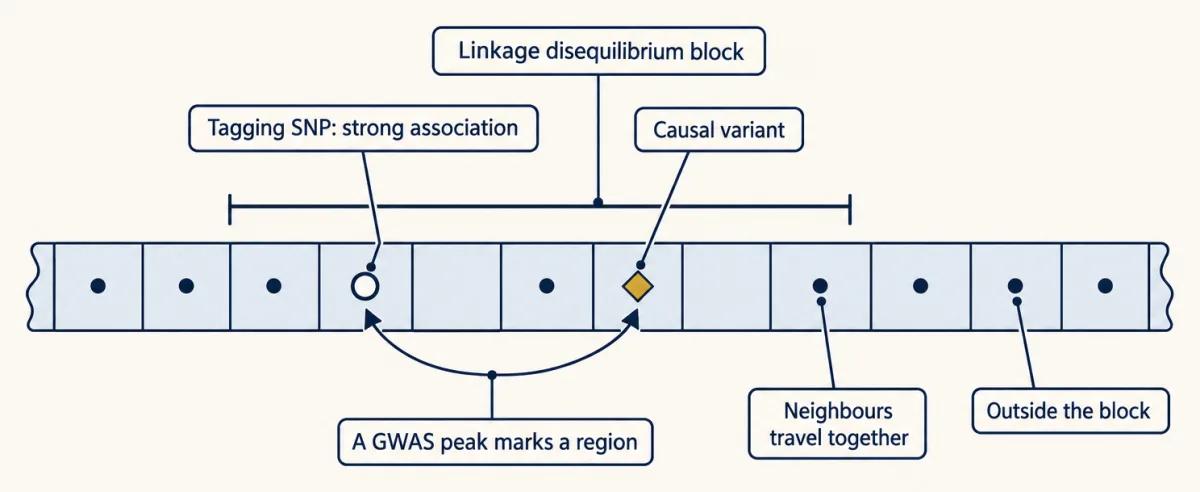
In 2005 Klein and colleagues, with 96 cases of age-related macular degeneration and 50 controls, found a strong association with a common intronic SNP in CFH, then proposed a coding change in LD with it as a candidate cause.
Predict. With twice as many independent tests, should the Bonferroni threshold be larger or smaller?
Worked problem 4. Why 5 x 10⁻⁸? Pe’er and colleagues estimated about one million independent common-variant tests across the genome in European-ancestry HapMap data. A Bonferroni correction divides the acceptable chance of any false positive, 0.05, by the number of tests: 0.05 / 1,000,000 = 5 x 10⁻⁸. In powers of ten, 0.05 is 5 x 10⁻² and a million is 106, and dividing subtracts the exponents: −2 − 6 = −8. Written out, that is 0.00000005 (see powers). The same study estimated about twice as many independent tests in African-ancestry HapMap data, where LD blocks are shorter. Twice the tests halves the threshold, to about 0.05 / 2,000,000 = 2.5 x 10⁻⁸. The threshold is a convention tied to those LD patterns.
A false hit can also come from population stratification, the second film’s ancestry imbalance: SNPs whose frequencies differ between the source populations can look associated even when they do not affect the trait. Price and colleagues showed in 2006 that principal components of genome-wide genotypes (a few summary axes of genetic variation that track ancestry) can model these differences; they are now standard covariates that reduce confounding without guaranteeing its absence.
Yang, Visscher and colleagues estimated in 2010 that common SNPs analysed jointly captured 45% of height variance in 3,925 unrelated people, far more than the significant hits alone, because most effects are too small to pass the threshold. Later whole-genome sequencing suggested that much of the remaining gap lies in rare variants that arrays tag poorly.
From a hit to a mechanism
The second film’s three rungs, fine-mapping, colocalization and editing, are tidier than a real locus. Fine-mapping often uses linkage disequilibrium (LD) patterns from several ancestry groups to build a credible set likely to contain the causal variant, and colocalization often points to a gene other than the nearest.
At FTO the work relied on chromatin contacts, epigenomic maps and editing more than on formal fine-mapping. The obesity association lies in FTO introns, yet Smemo and colleagues (2014) reported that the region regulates IRX3. Claussnitzer and colleagues (2015) then studied human fat-cell precursors and linked the signal to rs1421085, a T-to-C change that disrupts a binding motif for the repressor ARID5B and is associated with doubled IRX3 and IRX5 expression early in differentiation. Correcting the allele by CRISPR in cultured primary adipocytes from a risk-allele carrier restored heat production, reported as about sevenfold. That edit supports a cellular mechanism; it does not show weight change in a person. The mechanism is still debated: later work found several functional variants on the same haplotype, and mice carrying the risk base had more brown-fat heat production, not less. See the CRISPR lesson for the tools.
Polygenic scores, portability and the weight of history
A polygenic score sums weighted allele counts:
In words The polygenic score is, for every SNP in the panel, the effect estimate times how many copies of the effect allele the person carries, all added up.
- PGS“P G S, polygenic score”
- the person's score, in the trait's units (cm for height)
- effect estimate“effect estimate”
- the GWAS estimate of how much one copy of the allele shifts the trait, on average, in the study population
- allele count“allele count”
- how many copies of that allele the person carries: 0, 1 or 2
Sanity check Someone carrying no copies of any effect allele scores 0, and each extra copy adds its effect once. The effect estimates come from one study population, so the score is only as accurate as those estimates are for the person being scored.
Try one number
A made-up panel of three SNPs, to show the arithmetic: effects +0.5, +0.2 and −0.3 cm per copy; the person carries 2, 1 and 0 copies.
PGS = 0.5 × 2 + 0.2 × 1 + (−0.3) × 0 = 1.0 + 0.2 + 0 = 1.2 cm.
A real height panel sums thousands of such terms, each tiny.
A polygenic score must be tested outside its GWAS; accuracy can drop when linkage disequilibrium (LD), allele frequencies, effect sizes or environments differ. Like heritability, its accuracy belongs to the population and setting where it is tested. Yengo and colleagues reported in 2022 that their 12,111-SNP height panel captured about 40% of variance out of sample in European-ancestry analyses but around 10 to 20% in the other ancestry groups examined; they judged differences in LD and allele frequency likely explanations. Martin and colleagues reported in 2019 that the scores of that time were several times more accurate in European-ancestry individuals, and warned that clinical use could widen health disparities. Accuracy also varied with age, sex and socioeconomic characteristics within one ancestry group in UK Biobank, as Mostafavi and colleagues found in 2020. Allele frequencies are the subject of population genetics.
Genetic prediction has a history. Francis Galton coined the word eugenics in 1883. In the United States, states passed laws for forced sterilization of people judged unfit, and in Buck v. Bell (1927) the Supreme Court upheld Virginia’s law. Tens of thousands of people were sterilized. That history is why the second film’s three questions come before clinical use.
Design problem
Predict. Does p = 3 x 10⁻¹² pass a threshold of 5 x 10⁻⁸? Compare the exponents first.
A genome-wide association study (GWAS) reports a lead single nucleotide polymorphism (SNP) in an intron of gene A, with p = 3 x 10⁻¹² and an odds ratio of 1.08 per risk allele. The associated LD block spans genes A, B and C. In the relevant tissue, the risk allele associates with higher expression of C, not A. Which gene is causal, and how would you find out?
Saved in this browser only.
One way to do it
Do not name a gene from the association. The p-value (3 x 10⁻¹², below 5 x 10⁻⁸) says data this extreme would be very unlikely if the lead SNP had no association with the trait, not which variant or gene is responsible, because SNPs in strong LD with the lead SNP can carry a similar signal. An odds ratio of 1.08 is a small effect for any one person.
- Fine-map. Use the LD structure, ideally from cohorts of more than one ancestry, to build a credible set of variants likely to contain the causal one.
- Colocalize. Test whether the disease signal and the expression signal for C share one causal variant, rather than being two nearby signals; test A and B too.
- Edit. In the relevant human cell type, use CRISPR to swap the credible-set variant (or delete the candidate enhancer), with matched unedited and sham-edited controls. Measure A, B and C expression and a cellular phenotype linked to the disease.
The FTO region, though still debated, is the precedent. A positive edit implicates C in that cell type; linking C to the disease still needs evidence from whole organisms or human genetics.
Your notes
Select any text in the lesson to highlight it or add a note to it. Your highlights and notes are saved in this browser and collected in your notebook.
This browser is not letting the site save anything (a private window or strict privacy settings), so highlights and notes will be lost when you leave the page.
How we measure it
Classical twin design (ACE model)
Compare how similar identical (monozygotic) twins are with how similar fraternal (dizygotic) twins are for a trait. Under stated assumptions the difference estimates additive genetic variance (A), shared environment (C) and unique environment plus error (E).
Genome-wide association study (GWAS)
Genotype hundreds of thousands to millions of SNPs in many people, regress the trait (or case status) on allele dosage at each SNP with ancestry principal components as covariates, and keep SNPs that pass P < 5 × 10^-8. A hit marks a region, not a causal variant.
Fine-mapping and colocalization
Use the pattern of linkage disequilibrium to rank the variants in an associated region and define a credible set likely to contain the causal one. Then test whether the trait signal and a gene-expression signal in a relevant tissue share the same variant.
Polygenic score construction and evaluation
Sum each person's allele counts weighted by GWAS effect estimates, then measure how much variance the score adds to a covariate-only model in people who were not in the GWAS. The result holds only for the population and setting where it was measured.
Practice questions on this lesson (3) → MCAT-style, original, each with an explanation
Where this lesson fits
Before thisReview first
- Probability, Crosses and the Chi-Square TestThis course · Lesson 3
You need to multiply and add probabilities over independent allele draws to see why many loci give a bell curve.
- Population Genetics: Hardy-Weinberg and Evolutionary ForcesThis course · Lesson 25
Allele frequencies and what changes them underlie variance partitioning, linkage disequilibrium and why scores transfer poorly between groups.
- Extending Mendel: Dominance, Multiple Alleles and Gene InteractionThis course · Lesson 4
Dominance, gene interaction and incomplete penetrance are the sources of the non-additive variance partitioned here.
After thisStudy next
- Molecular EvolutionEcology and Evolution · College: the core
This course's variants and allele frequencies carry on into how sequence differences build up between species.
- How to Test an Evolutionary ExplanationEcology and Evolution · College: the core
It takes heritable variation further, asking when selection on a trait counts as evolution.
Elsewhere on the siteFilms, simulations and method films in other courses
- Experimental units, pseudoreplication and powerMethod film
Choosing the true unit and sample size matters when planning an association study and judging its significance threshold.
Suggested by an AI model from the lessons themselves, then checked. How we use AI
Finish line
Test yourself
8 questions
Practice and MCAT-style, with explained answers.
That's the last lesson · Next course
Ecology and Evolution
How populations change over generations, and how organisms, populations and ecosystems work together.
Start the next course →Before you move on: review the questions you missed , or go back to all lessons in this course.
← Lesson 25 · Population Genetics: Hardy-Weinberg and Evolutionary Forces