Neuroscience · Unit 7: Evidence and disease
Recording Many Neurons: Imaging, Arrays and Atlases
Rewritten on : new text, figures, flashcards and film. Your notes and highlights stay, but the text around them may have moved.
A probe with 960 recording sites does not record one neuron per site. What does it record?
Pause when the reading reaches a film, and offer to play it. Saved on this device.
Watch the film now, or keep listening
Builds on:The Action Potential and ConductionPrinciples of Sensory CodingWhy these?
 ▶ Watch One Question for Every Number · 2:17
Read the transcript of “One Question for Every Number”
Film transcript: One Question for Every Number
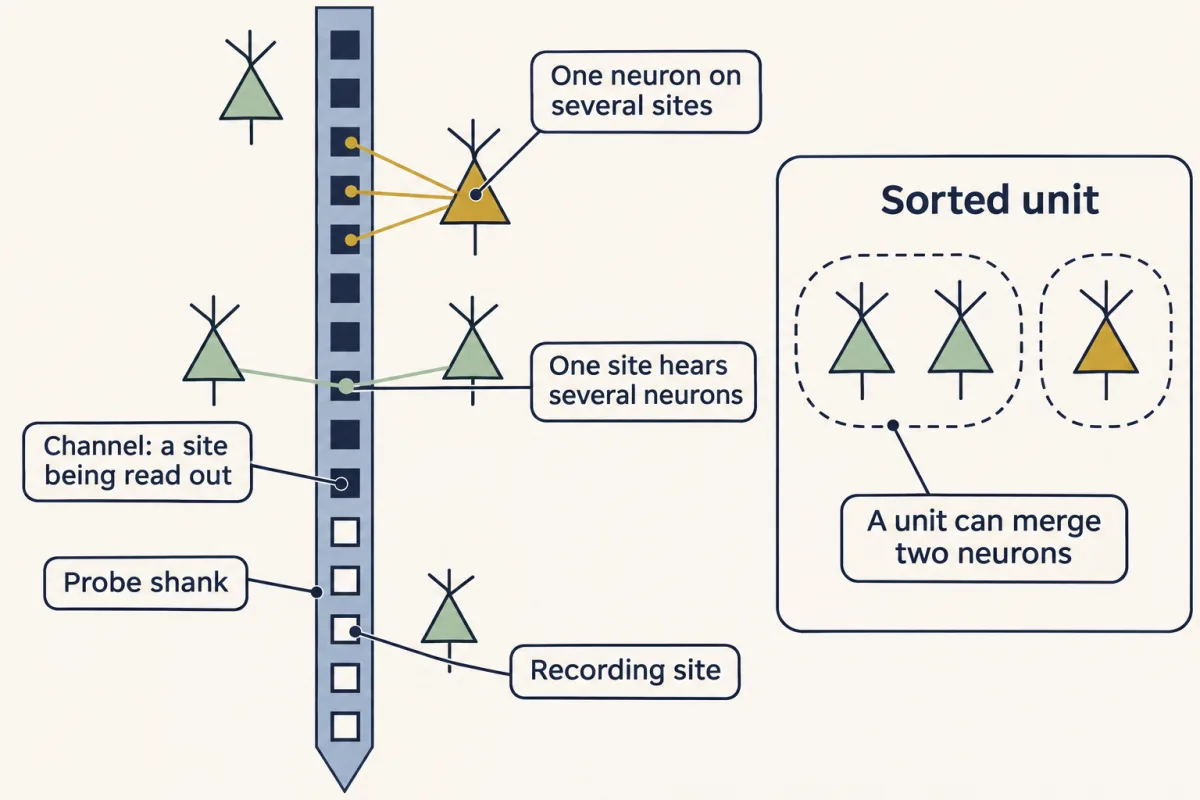
The original Neuropixels probe carries 960 recording sites. Does it record 960 neurons? Not necessarily. The original probe reads out only 384 sites at a time. Each one read out is a channel. And neurons are not read off sites at all. Software sorts the spikes into units. It can find more units than channels, or fewer. One neuron shows up on several neighbouring sites. One site hears several neurons. So a unit can merge two neurons, or split one. Treat each unit as an inference, with quality scores. Notice the ladder. Sites, then channels, then units, then neurons. Each rung is a step from what you want. Calcium imaging has a ladder too. A spike lets calcium in, and calcium makes a sensor glow.
The glow is real, but it lags and blurs the spike, like steam from a kettle. An atlas sorts cells into clusters. Is each cluster a true cell type? Not every one may be. A connectome counts synapses. Is a count a strength? Treating it as one is an assumption, not a measurement. Even a pile of units has a step. Units from one mouse share that mouse. So here is the one idea. Each of these numbers is a proxy, one or more steps from your claim. Name each step. Trust it only as far as someone has measured that step, in conditions like yours. More cells sharpen the estimate for each animal. But they never count as more animals. Every method has a row like this: the number it gives, and the step to your claim.
The rule says how far to trust a measurement. It cannot show a pathway is needed. That takes a manipulation. The next two films follow two of these steps closely: light to spikes, and cells to mice.
From the film
- Each big number in large-scale neuroscience is a proxy, one or more steps from your claim.
- Trust each step only as far as someone has measured it in conditions like yours.
- More cells sharpen the estimate for each animal, but they never count as more animals.
- The rule says how far to trust a measurement, not whether a pathway is needed for anything; that takes a manipulation.
The original Neuropixels probe (2017) carries 960 recording sites along one shank about 10 mm long. Push it into a mouse brain and you can hear spikes from hundreds of neurons at once.
That is a long way from one electrode in one cell, and other methods have scaled up too: calcium imaging films the glow of hundreds of identified neurons, transcriptomic atlases sort millions of cells into types, and connectomes trace the chemical synapses of a whole piece of brain. Each method hands you a big number that, taken at face value, can lead you to a wrong conclusion. This lesson asks what each one actually counts.
Four big numbers, four questions
Each number sounds like the thing you want to know, and each hides a question.
- Sites. A probe has 960 recording sites. Does it record 960 neurons?
- Glow. A neuron glows brighter for a moment. How many spikes did it fire?
- Units. A study records 300 units from three mice. How many samples does it have?
- Synapses. A wiring diagram shows 50 synapses from neuron A onto neuron B. How strongly does A drive B?
In every case the starting number alone does not answer the question. You need to know what was measured and justify each step from that measurement to your claim.
The one idea to carry through this lesson. Each big number in this lesson is a proxy, one or more steps away from the thing your claim is about. Name each step, and trust it only as far as someone has measured that step in conditions like yours. Going from many cells to “mice in general” is one of those steps too, a step of sampling rather than of instruments: more cells sharpen the estimate for each animal, but they never count as more animals.
The rule applies to observational datasets, of activity (imaging and probes) and of anatomy (atlases and connectomes). It tells you how far a measurement can be trusted, not whether a pathway is needed for anything; that takes a manipulation, the subject of designing a circuit experiment.
Skim the table now; each section of the lesson fills in one row.
| Method | What it gives you | The step to your claim | What checks the step |
|---|---|---|---|
| High-density probe | sorted units | sites → channels → units → neurons | quality scores, only partly; a unit can still merge or split neurons |
| Calcium imaging | ΔF/F0, a change in light | light → calcium → spikes | a simultaneous electrical recording, valid only for the conditions tested |
| Any recording | many units and trials | units → animals | analysis at the animal level; more units sharpen each animal’s estimate, but only more animals add samples |
| Transcriptomic atlas | clusters of cells | cluster → cell type | partly, by matching clusters to anatomy; the authors say some clusters may not be true types |
| Connectome | synapse counts | count → strength and sign | not measured by the connectome; treating count as strength is an assumption |
Probes: sites, channels and units
Predict. A Neuropixels probe has 960 recording sites. Will it record 960 neurons at once, more, or fewer? What would you need to know to answer?
Check your prediction
Not necessarily 960, and there is no fixed number. The original probe’s electronics (Jun and colleagues, 2017) could read out only 384 of its sites at once (the experimenter picks which, within limits set by the wiring), digitizing the action-potential band at 30 kHz, a sampling rate, not a firing rate. Each site being read out is a channel. And neurons are not read off sites at all: software has to sort the spikes into units, and it can find more units than channels or fewer. With two probes in an awake mouse, 768 channels in all, the team recorded more than 700 well-isolated neurons at once across five brain structures, in the same range as the channels but reached by sorting. The count depends on where the probe sits and on how the spikes are sorted.
An extracellular electrode sits outside cells and picks up the small voltage changes that nearby spikes cause in the surrounding fluid, unlike the intracellular recordings in the resting membrane and passive signals. It loses the membrane potential but keeps millisecond timing.
Sites and channels, the first two rungs of the probe’s ladder, are hardware. The next rung is an inference. Spike sorting software detects spikes and groups them into units by the shape of each spike and the sites where it appears. One neuron shows up on several neighbouring sites; one site hears several neurons. So a unit can merge two neurons or split one. Even a “well-isolated” unit is a judgment made from quality scores: treat it as an inference, not as a confirmed single neuron. The Allen Institute’s documentation for its own Neuropixels survey warns that spikes from different neurons can be mixed in one unit, and that it does not separate single-unit from multi-unit activity.
Imaging: light, two steps from a spike
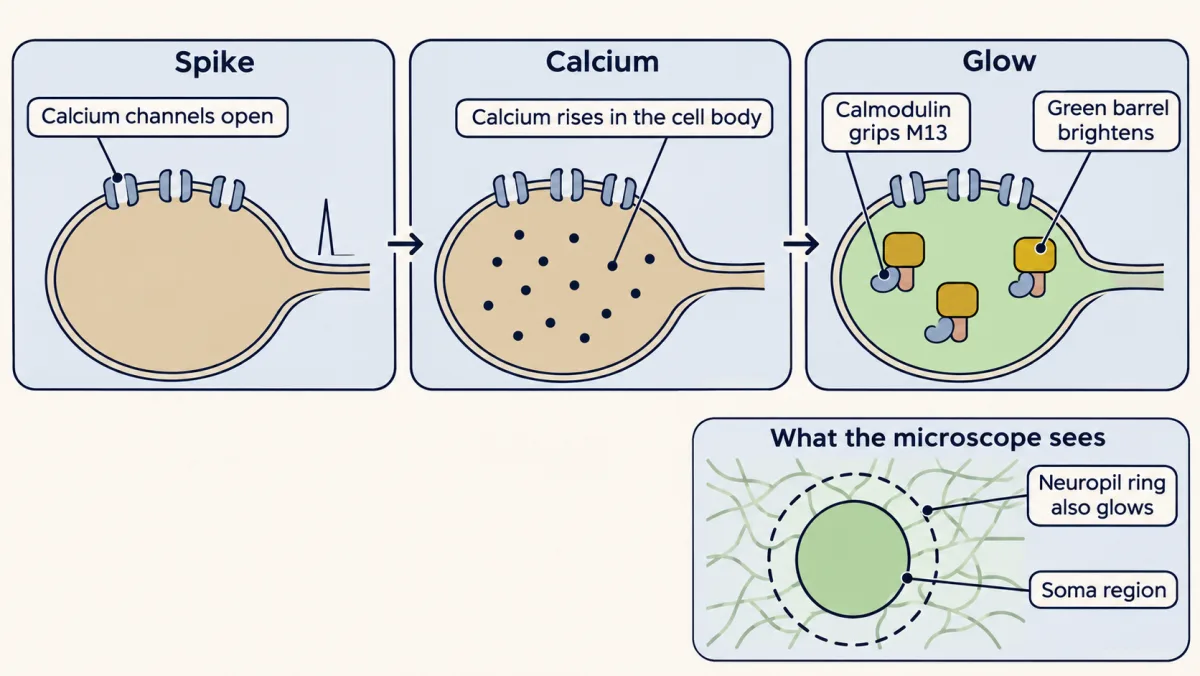
When a neuron fires an action potential, voltage-gated calcium channels open and calcium in the cell body rises for a while after the spike. A genetically encoded sensor turns that rise into light. GCaMP6 is one protein that joins a green fluorescent protein to calmodulin, the calcium-binding protein you met in calcium signaling. Calcium-bound calmodulin grips a short peptide, M13, built into the same protein, and that change of shape makes the green barrel brighter. The structures panel shows the parts. How the sensor is delivered, by virus or by a transgenic mouse line, belongs to hacking the cell, and how a two-photon microscope collects the light belongs to microscopy and images.
So the light is two steps from the spike: the spike lets calcium in, and calcium makes the sensor glow. A spike is over within a few milliseconds, but the calcium and the glow it causes rise and fade far more slowly. It is like reading a kettle’s steam to infer when the stove was switched on: the steam is real, but it lags and blurs the moment you care about.
Activity is reported as a fractional change from baseline:
ΔF/F0 = (F − F0) / F0
F is the fluorescence at one moment and F0 is the baseline. Dividing by the baseline cancels a brightness scale shared by baseline and response, such as laser power or how much sensor the cell makes, once background light has been removed. It does not make cells fully comparable: expression also changes calcium buffering, and photon noise still differs.
The neuropil problem
Around each cell body lies neuropil, the dense tangle of axons, dendrites and glial processes; its axons and dendrites carry the sensor too, so it also glows. Light from it leaks into any region you draw around a soma. The usual fix subtracts a scaled copy of the surrounding signal:
F_corrected = Fsoma − r × Fneuropil
Worked problem. These numbers are invented for practice. A soma region reads 500 at baseline and 620 at the peak (arbitrary units). The ring of neuropil around it reads 300 and 330.
Step 1: no correction. ΔF/F0 = (620 − 500)/500 = 120/500 = 0.24.
Step 2: subtract neuropil. Take r = 0.8, the default that Huang and colleagues (2021) used in mouse visual cortex; they adjusted it for some cells, so it is not a universal constant. Then F0 = 500 − 0.8 × 300 = 500 − 240 = 260, and F = 620 − 0.8 × 330 = 620 − 264 = 356.
Step 3: recompute. ΔF/F0 = (356 − 260)/260 = 96/260 = 0.37.
The correction raised ΔF/F0 by about half. Assumptions: r is the same at baseline and peak, and the neuropil ring samples the same contaminating light as the soma.
Predict. Does subtracting neuropil always raise ΔF/F0? Keep the soma at 500 and 620, but suppose the neuropil ring had brightened more during the response, from 300 to 390.
Check your prediction
No. It depends on which brightened more, in proportion. The soma rose by 24% (120 on 500).
- Neuropil 300 → 330, a 10% rise (the worked problem): 0.37, higher than 0.24.
- Neuropil 300 → 372, a 24% rise: F = 620 − 297.6 = 322.4, so ΔF/F0 = 62.4/260 = 0.24, no change.
- Neuropil 300 → 390, a 30% rise: F = 620 − 312 = 308, so ΔF/F0 = 48/260 = 0.18, lower than 0.24.
The rule: with r above zero and a corrected baseline that stays positive, the correction raises ΔF/F0 when, and only when, the neuropil’s fractional change is smaller than the soma’s. In the worked problem it was, because the neuropil had added a large, nearly steady glow to the baseline.
How many spikes is a flash? Calibrate it
Read the transcript of “The Answer Key: How Many Spikes Is a Flash?”
Film transcript: The Answer Key: How Many Spikes Is a Flash?
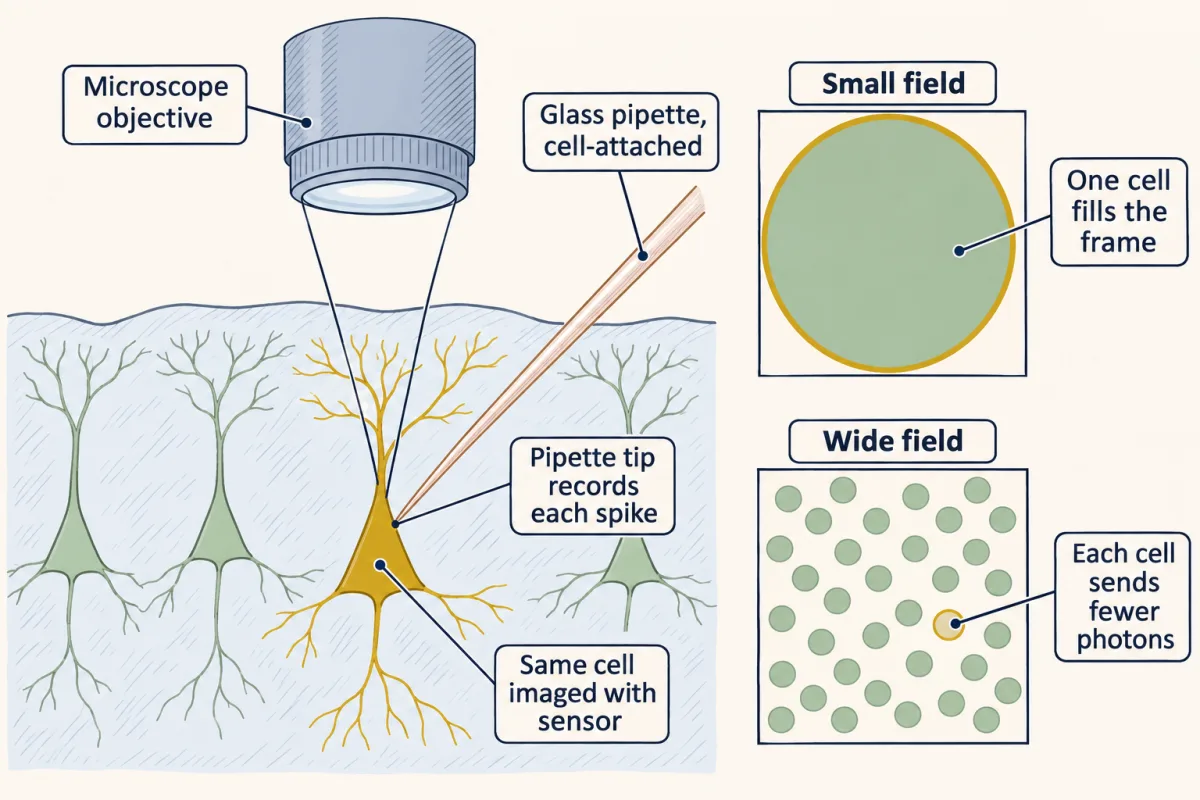
A neuron flashes brighter for a moment. How many spikes did it fire? The glow is measured in light, not spikes. To translate, record both at once in a sample of neurons. Then ask whether that calibration fits your conditions. A fine glass pipette presses against the outside of the cell, without breaking in. It picks up each spike electrically. This is a cell-attached recording. Meanwhile, the microscope films the same cell's glow. Picture the record. Spike ticks from the pipette run along the top, and the glow runs below. The spikes are the answer key. You ask how often the light gets them right. The detection rate is the fraction of isolated single spikes that the light reveals.
The false-positive rate is the fraction of spike-free test windows in which the light reports a spike anyway. You can always find more spikes by accepting more false alarms. So fair comparisons fix the false alarms at 1% % of spike-free windows. First, the best case. Chen and colleagues made detection as easy as possible, with a magnified view of one cell. The sensor, GCaMP6s, revealed nearly every isolated spike. Now widen the field to hold hundreds of cells. Each cell becomes a tiny part of the picture. What happens to single-spike detection, and why?
It falls further. Huang and colleagues repeated the calibration in transgenic mice. Even at high magnification, their tuned detector caught fewer single spikes than in Chen's cells. The authors proposed weaker expression and more labelled neuropil as possible reasons. When the movies were made to mimic a wide field, it caught only a minority. Standard software without the answer key often caught under one spike in ten, even before that. Huang and colleagues pointed to photons. A wider field spreads the imaging time over more pixels. Each neuron sends back fewer photons. Photon counts flicker at random, and one spike's glow sinks into the flicker.
If the cell sends back the same photons per second, a slower frame rate costs a slow sensor little. Frame rate still limits spike timing. So a calibration belongs to its conditions, not to the sensor. Before turning glow into spikes, ask: was it calibrated at your field of view, expression level and cell type? And in population imaging, a flat trace does not prove a silent cell. One or a few spikes can hide in it.
From the film
- Fluorescence is measured in light, not spikes, so turning it into spikes needs a calibration against an electrical recording of the same cells.
- A calibration belongs to its conditions, not to the sensor, so ask whether it was done at your field of view, expression level and cell type.
- In population imaging a flat trace does not prove a silent cell, because one or a few spikes can hide in it.
A ΔF/F0 trace is measured in light, not in spikes. To translate one into the other you need a dictionary. You write it by recording both at once from a sample of neurons, then ask whether that calibration fits your conditions; it gives an estimate with error, not an exact lookup. In a loose-seal cell-attached recording, a fine glass pipette pressed against the outside of the cell, without breaking in, picks up each spike electrically while the microscope films that cell’s fluorescence. The electrical record is the answer key, and you ask how often the light gets it right.
Picture the record: a row of spike ticks from the pipette on top, the ΔF/F0 trace of the same cell below, on one time axis. Two numbers score the light against the ticks. The detection rate is the fraction of isolated single spikes that the light reveals. The false-positive rate is the fraction of designated spike-free test windows, of a length set by each analysis, in which the light reports a spike anyway: at 1%, about one such window in 100. It is not the fraction of reported spikes that are wrong. You can always find more spikes by accepting more false alarms, so fair comparisons fix the false-positive rate, here at 1%, and compare detection rates.
The best case. Chen and colleagues (2013) set up mouse primary visual cortex to make detection as easy as possible: layer 2/3 pyramidal neurons in lightly anesthetized, sedated mice, GCaMP6s expressed from a virus, high-magnification imaging of the recorded cell and a stimulus adjusted to keep firing moderate. GCaMP6s detected 99 ± 0.2% of isolated spikes at a 1% false-positive rate, in nine cells.
Predict. Now image the way a population experiment does, with a field of view wide enough to hold hundreds of cells. Each cell is now a tiny part of the picture. What happens to single-spike detection, and why?
Check your prediction
It falls further. Huang and colleagues (2021) repeated the calibration in anesthetized transgenic GCaMP6s and GCaMP6f mice, keeping 48 neurons in their final set. Even at high magnification (a small field centred on each soma at about 158 frames per second), a detector tuned to each neuron’s known spike times caught fewer single spikes than in Chen’s cells, about 40 to 80% on average depending on the mouse line. That first gap is not about field of view: the authors proposed weaker transgenic expression and more labelled neuropil as possible reasons. They then downsampled the movies to the pixels and frames of a 412 by 412 µm field at 30.3 frames per second, and the tuned detector caught only about 16 to 43% (32 to 43% in the GCaMP6s lines, less in the faster GCaMP6f lines). At the same 1% false-positive rate, standard blind spike inference, which does not know the answer key, often caught fewer than 10%, even before downsampling.
The explanation Huang and colleagues gave is photons. A larger field of view spreads the same imaging time over more pixels, so each neuron sends back fewer photons. Photon counts flicker at random, and the small glow from one spike sinks into that flicker. For a slowly decaying GCaMP6s transient, dropping from about 158 to 30 frames per second costs little in a simple model, as long as the cell sends back the same photons per second. Frame rate still limits spike timing and matters more for fast sensors and overlapping events (Going deeper has a rough estimate).
So a calibration belongs to its conditions, not to the sensor. Before you turn ΔF/F0 into spikes, ask whether anyone has calibrated it at your field of view, your expression level and your cell type. The spike-to-fluorescence relation also differs from one neuron to the next. GCaMP6s decays slowly, and the fast GCaMP6 variants trade sensitivity for speed. Newer sensors such as jGCaMP8 respond more linearly than earlier GCaMPs, but none of them reports voltage, and none removes the need for an answer key. In population imaging a flat trace does not prove a silent cell: one or a few spikes can hide in it.
Two methods, two ladders
Imaging tells you which cell, where, and often its genetic type, but its light is slow and two steps from the spike. Probes give millisecond spike timing across many regions, as in the Allen Institute’s survey of six cortical and two thalamic visual areas in mice (Siegle and colleagues, 2021), but the identity of each unit is uncertain. The codes these populations carry are the subject of sensory coding and the visual cortex.
How many samples do you really have?
Read the transcript of “How Many Mice?”
Film transcript: How Many Mice?
300 units, recorded from 3 mice. How many samples is that? Units recorded from one mouse share that mouse: its genes and its drug dose. Units recorded in one session also share that day's alertness, and one probe track. If that mouse or session is unusual, its units tend to shift together. Take a small invented dataset. Two mice. Mouse A gave four units, and mouse B gave two. Pool every unit, and mouse A counts twice as much, only because it gave more units. Average within each mouse first, and each animal counts once. The animal mean comes out lower.
For a claim about mice, the sample is 2, not 24. Now a harder test. Suppose a drug does nothing at all, on average. Record 100 units from each of 3 mice. Treat all 300 as independent. How often will a standard test call the drug effect significant?
In a simulation with invented numbers, about 7 times in 10. The same test on the 3 mouse averages was significant only about 5 times in 100. That is the false-alarm rate the test is built to give, when its assumptions hold. Counting units as independent made the error bars far too narrow. This is called pseudoreplication. Are more units worthless, then? No. They average out the noise between units within each mouse. But no number of units averages out the differences between mice. The error stops shrinking at a floor. With the spread between mice held fixed, only more mice lower the floor.
So report every level, and say which level your question is about. Each of these numbers is a step from your claim. Count your sample at the level of the claim. And none of this shows that a pathway is needed. That takes a manipulation.
From the film
- Units recorded from one mouse share that mouse, so counting them as independent samples is pseudoreplication.
- For a claim about mice, the sample is the number of mice, not the number of units.
- More units sharpen each mouse's estimate, but only more mice lower the floor on the error.
Large datasets are nested: units within sessions, sessions within animals. Within a session, every unit recorded together sees the same stimulus presentations, so each unit–trial pair is one observation. Units from one mouse share its genes and its drug dose; units recorded in one session also share how alert it was that day and the track of one probe. If that mouse or session happened to be unusual, its units tend to shift together. Observations that share conditions like this are not independent, and counting them as if they were is pseudoreplication (Lazic, 2010). The fix is to analyse at the level of your claim: average within each animal (one way Lazic describes to keep animals as the units of analysis), or use a hierarchical (mixed-effects) model, which estimates the variation between animals and within them separately.
Worked problem. This dataset is invented. Two mice, A and B, each have two sessions. In each session the same stimulus is shown four times, and spikes are counted in a 0.25 s window per presentation. Each unit appears in one session only.
- Mouse A, session 1: U1 (1, 2, 3, 2) and U2 (0, 0, 1, 1)
- Mouse A, session 2: U3 (1, 1, 1, 1) and U4 (2, 2, 2, 2)
- Mouse B, session 3: U5 (0, 1, 0, 1)
- Mouse B, session 4: U6 (1, 0, 1, 0)
Step 1: count. 6 units, 4 sessions, 2 animals, 6 × 4 = 24 unit-trials, but only 4 × 4 = 16 stimulus presentations.
Step 2: rates. Each unit is watched for 4 × 0.25 s = 1 s. U1 fired 1 + 2 + 3 + 2 = 8 spikes, so 8 spikes/s. The six rates are 8, 2, 4, 8, 2 and 2 spikes/s.
Step 3: pooled rate. 26 spikes over 6 unit-seconds = 4.33 spikes/s.
Step 4: weight each animal equally. Session 1 averages (8 + 2)/2 = 5 and session 2 averages (4 + 8)/2 = 6, so mouse A = 5.5 spikes/s. Sessions 3 and 4 each give 2, so mouse B = 2 spikes/s. The animal mean is (5.5 + 2)/2 = 3.75 spikes/s.
The pooled rate is higher because mouse A supplied twice the units. For a claim about mice, n = 2, not 24.
Predict. A drug does nothing on average. You record 100 units from each of three mice before and after giving it, and run a t-test that treats all 300 units as independent. At the usual 5% threshold, how often will the test call the drug effect “significant”?
Check your prediction
About 7 times in 10. In a simulation with invented numbers (the model is in Going deeper), each mouse’s units shifted together by a random amount, as if that mouse’s state or probe track differed, and units varied among themselves with a standard deviation twice that of the mice. A two-sided t-test on the 300 units’ before-after changes was “significant” in 68% of 300,000 simulated experiments. The same test on the three mouse averages was significant in 5%, the nominal false-alarm rate, which holds here because the model meets that test’s assumptions. Because each mouse’s units move together, 300 units carry not much more information about the drug than three mouse averages do, yet the test counts 300 independent samples, so its error bars were far too narrow.
Does that make more units worthless? No. More units average out the unit-to-unit noise within each mouse, so each mouse’s average gets sharper. But they cannot average out the differences between mice: with that spread held fixed, the error stops shrinking at a floor that only more mice lower. Report the hierarchy (animals, sessions, units, trials) and say which level your question is about.
- Mean at this level
- n at this level
- Pooled rate (all units)
- Animal mean (mice weighted equally)
In this sketch: invented counts (spikes in 0.25 s windows, four presentations per session), each unit in one session only, means without spread.
Counting units or trials as independent is pseudoreplication (Lazic, 2010); averaging within animals, or a mixed-effects model, keeps the animal as the unit. Say which level the question is about.
Atlases and connectomes: steps the data do not fully check
The last two rows of the table are anatomy, not activity, and in both the final step is not fully measured by the dataset itself.
An atlas turns gene expression into a list of clusters. The step from cluster to cell type has not been fully tested. A transcriptomic atlas sorts cells by the RNA they express; a cluster is a group of cells whose expressed genes are similar. Yao, Zeng and colleagues (2023) profiled around seven million cells from the adult mouse brain, kept the roughly four million that passed quality control, and sorted them into 5,322 clusters. A spatial dataset, a 500-gene panel measured by MERFISH in about 4.3 million cells from one male mouse brain, placed the clusters back in the anatomy, and transcriptomic identity and location matched to a high degree. The sequencing itself is taught in sequencing and genomes. The authors cautioned that not every cluster may be a true cell type, and that dissociation (separating tissue into single cells for sequencing) probably depletes large, fragile neurons. A cluster is a molecular category, not a measured function.
A connectome counts synapses; it does not measure strength or sign. A connectome is a synapse-by-synapse wiring diagram. FlyWire (Dorkenwald and colleagues, 2024) reconstructed 139,255 neurons and 54.5 million chemical synapses from serial-section electron micrographs (the tissue cut into thin slices, each imaged) of one adult female Drosophila brain. A connection from neuron A to B is the set of A’s synapses onto B. Electrical synapses (gap junctions) are absent from the map, and some connections of only a few synapses were missed.
Predict. Suppose a connectome shows neuron A making 50 synapses onto neuron B and 5 onto neuron C. Does A drive B ten times as hard as it drives C?
Check your prediction
The anatomy alone cannot say. Strength depends on release probability, receptor type and the sign of the transmitter, and a synapse count measures none of them. (FlyWire predicts transmitter identity from the images, but does not measure it.) Some models built on the connectome assume that strength is proportional to synapse count; that is an assumption, not a measurement. What the count does support is that A has a chemical path by which it could influence B, and C.
MICrONS: one cell, seen twice
In one awake mouse, the MICrONS Consortium (2025) recorded calcium signals from around 75,000 neurons in visual cortex over a week of imaging sessions, then reconstructed the same tissue by electron microscopy: more than 200,000 cells and half a billion synapses. The imaged neurons were excitatory neurons expressing GCaMP6s across primary and higher visual areas. About 15,000 reconstructed neurons were matched by hand to their imaged responses.
In the terms of this lesson’s rule, MICrONS narrowed one gap: for the matched neurons, the imaged response and the reconstructed wiring can be assigned to the same cell, though the matching is itself a step that can err. The other steps remain. The light is still two steps from the spikes, a synapse count is still not a strength, and the whole dataset is still one mouse and about one cubic millimetre of cortex.
What none shows alone
Each method answers a different question. Imaging says which cells changed their calcium; probes say when units spiked; atlases say what molecular kinds of cells exist and where; connectomes say who could talk to whom. None of the datasets here is human, none is a complete brain map with activity and strengths, and none shows that a pathway is needed for a behaviour; that still takes a manipulation.
Design problem
A lab images 400 neurons in mouse V1 in three mice with GCaMP6s at 30 frames per second over a wide field of view. It reports that 60% of the neurons “did not fire” to a visual stimulus, and cites the connectome of a different mouse showing few thalamic synapses onto those cell types. Critique the claims and redesign the study.
Saved in this browser only.
One way to do it
The imaging claim. No fluorescence change is not the same as no spikes. Under wide-field, population-like conditions, Huang’s calibration detected only a minority of single spikes, often under 10% with blind spike inference. Calibrate in this preparation: record cell-attached spikes from a sample of neurons while imaging at the same field of view and frame rate, and report detection and false-positive rates. A Neuropixels probe in the same area adds millisecond spike timing, but in a standard preparation its units usually cannot be matched one to one to the imaged cells, and it can miss neurons that rarely fire.
The statistics. The 400 neurons come from three mice, so n = 3 for any claim about mice. Report the fraction per mouse and add animals.
The anatomy. The connectome is from one other animal, contains chemical synapses only, and counts synapses rather than measuring strength. Few synapses do not mean weak drive. Either register function and structure in the same tissue, imaging first and reconstructing afterward as MICrONS did, or test the input directly: stimulate the thalamic afferents, for example optogenetically, and record the V1 neurons’ responses with calibrated imaging or a probe.
Going deeper
How GCaMP is built
The green fluorescent protein in GCaMP6, as in earlier GCaMPs, is circularly permuted: its ends have been reopened near the light-emitting chromophore, so the calmodulin and M13 domains can change the chromophore’s surroundings. The jGCaMP8 sensors (Zhang and colleagues, 2023) swap M13 for a peptide from another calmodulin-binding enzyme.
Photons, not frames: a rough estimate
This toy estimate assumes a fixed laser power sweeping the whole field evenly in the same total time, so the share of scan time spent on the soma equals the share of the field it covers. The sizes are illustrative, and it is not a reconstruction of Huang’s experiment. A soma about 12 µm across fills about 12.6% of a 30 µm field but only about 0.067% of a 412 µm field, so it sends back roughly 190 times fewer photons. In a simple model of photon noise, the single-spike signal-to-noise ratio scales with the square root of the photons collected, so it falls by about 14 times; detection probability does not fall in the same proportion. The same model predicts almost no change from the frame rate alone, but only for slow, isolated transients (a decay time of 0.1 s or longer in the model): simulated at 158 and 30.3 frames per second with the same photons per second from the cell, the signal-to-noise ratio was about the same.
How much do more units help?
Here is the invented two-level model behind the simulation. Each unit’s value (in the simulation, its before-after change) is a mouse effect plus a unit residual, all independent and normally distributed: mice differ with a standard deviation of 1, units within one mouse with a standard deviation of 2. The simulation used 3 mice with 100 units each, a true effect of zero, and two-sided one-sample t-tests against zero at 5%. Across 300,000 simulated experiments the false-positive rate was 67.8% with units as n and 5.0% with the three mouse means (NumPy default_rng seed 20261102, batches of 1,000, mouse shifts drawn before residuals). These rates belong to this model, not to every 3-mouse, 300-unit study. With 3 mice, the standard error of the grand mean is 1.29 with 1 unit per mouse, 0.68 with 10 and 0.59 with 100. With the variances held fixed it can never fall below 0.577 (the mouse SD divided by √3), however many units you add; with 12 mice the floor drops to 0.289.
Your notes
Select any text in the lesson to highlight it or add a note to it. Your highlights and notes are saved in this browser and collected in your notebook.
This browser is not letting the site save anything (a private window or strict privacy settings), so highlights and notes will be lost when you leave the page.
How we measure it
Two-photon calcium imaging
A genetically encoded sensor such as GCaMP is expressed in neurons, and a two-photon laser scans the tissue to measure each cell's fluorescence over time. It reports calcium, which rises after spikes, for hundreds or thousands of identified cells, but spike times must be inferred through a calibrated model.
High-density extracellular recording and spike sorting
A silicon probe such as Neuropixels records voltage from hundreds of sites along a shank. Spike-sorting software detects spikes and groups them into units by waveform and position, giving millisecond timing across many brain regions, with each unit an inference rather than a confirmed single neuron.
Single-cell RNA sequencing and spatial transcriptomics
Dissociated cells are sequenced one by one and clustered by gene expression; an imaging method such as MERFISH then measures a chosen gene panel in intact sections to place the clusters in the anatomy.
Serial-section electron microscopy connectomics
Tissue is cut into thousands of thin sections, each is imaged by electron microscope, and software with human proofreading traces neurons and marks chemical synapses through the stack. The result is a wiring diagram of one piece of tissue from one animal, with no record of activity.
Practice questions on this lesson (3) → MCAT-style, original, each with an explanation
Where this lesson fits
Before thisReview first
- The Action Potential and ConductionThis course · Lesson 4
You need to know what a spike is and how it lets calcium in before asking what probes and light record.
- Principles of Sensory CodingThis course · Lesson 9
Population recordings and sorted units are used there to read codes, so you need what a spike train carries.
After thisStudy next
- Designing a Causal Circuit ExperimentThis course · Lesson 28
Observational datasets cannot show a pathway is needed, so you take this idea further with a manipulation and its controls.
Elsewhere on the siteFilms, simulations and method films in other courses
- Extracellular single-unit and nerve recordingMethod film
It shows how spikes are picked out from outside the cell, the basis of sorted units on a probe.
- Before the Data ArriveFilm · Cell Biology
It shows why the independent unit must be fixed before data arrive, the same issue as units versus animals.
- What Zoom Cannot RecoverFilm · Cell Biology
It shows what image resolution can and cannot recover, relevant to reading fluorescence signals.
Suggested by an AI model from the lessons themselves, then checked. How we use AI
Finish line
Test yourself
8 questions
Practice and MCAT-style, with explained answers.
Next · Lesson 28
Designing a Causal Circuit Experiment
Light alone changed firing and turning behaviour in mice with no opsin at all. What does your light-on versus light-off comparison actually show?
Continue →