Neuroscience · Unit 7: Evidence and disease
Designing a Causal Circuit Experiment
Light alone changed firing and turning behaviour in mice with no opsin at all. What does your light-on versus light-off comparison actually show?
Pause when the reading reaches a film, and offer to play it. Saved on this device.
Watch the film now, or keep listening
Builds on:Emotion and StressRecording Many Neurons: Imaging, Arrays and AtlasesWhy these?
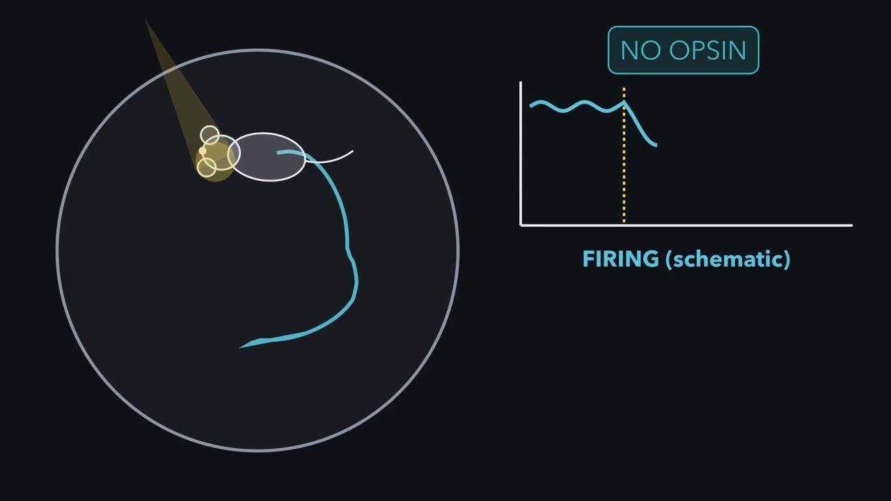 ▶ Watch What Did the Light Change? · 3:18
Read the transcript of “What Did the Light Change?”
Film transcript: What Did the Light Change?
A mouse has no opsin, yet light changes its firing and turning. What did the light change? In wild-type mice, continuous striatal light suppressed firing and biased turning. Illumination had changed tissue without a light-sensitive construct. A light-on comparison therefore changes at least two things: the intended neural activity and the light itself. A recording can show that activity and behaviour vary together. A manipulation asks a different question.
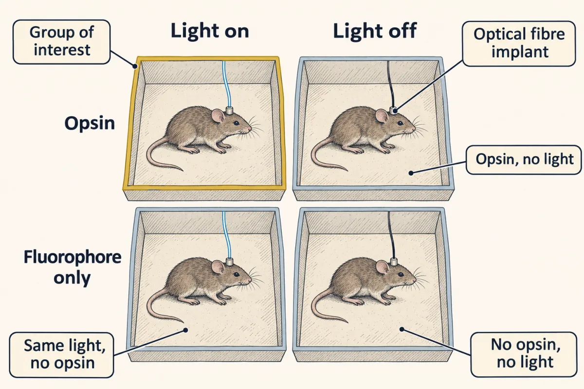
Driving chosen cells tests whether their activity is sufficient for the measured change. Suppressing them tests whether it is necessary. Each answer belongs only to the tested conditions. To separate the two causes, cross construct with light. Put opsin and fluorophore-only animals in two rows. Put light off and light on in two columns. Now every effect of illumination has a matched place to appear. You have compared light on with light off only in opsin animals. Which missing comparison would reveal whether light itself moved the behaviour?
Give fluorophore-only animals the same light. First measure the light effect in each row. Then compare those two effects. The shared light effect cancels. The remainder is the extra light-linked effect associated with carrying the opsin. Read the board as two differences, not four separate boxes.
Measure the light effect in opsin animals. Measure it again in fluorophore animals. Subtract the second effect from the first. This difference of differences identifies the opsin-linked remainder. That remainder is not a license to say the circuit controls the behaviour. Name the cells, the projection, the time window and the assay.
Activation tests sufficiency. Silencing tests necessity. Neither says these cells are the only route. A light spot does not name a pathway by itself. Terminal illumination can also excite labelled axons that only pass through the field. It can drive activity back toward the parent cell bodies. A local receptor block tests whether transmitter action there is required for the measured behavioural effect. Finally, verify what the manipulation actually did.
Record during and after the light. Confirm expression and fibre placement. Randomize allocation and blind the scoring. Only when the manipulation and its controls work can the matched contrast identify the effect. A claim can be no broader than that contrast.
From the film
- Light can change firing and behaviour even when no opsin is present.
- Driving activity tests sufficiency; suppressing it tests necessity under the tested conditions.
- Crossing construct with light separates an opsin-linked effect from an effect of light itself.
- A causal claim must name the cells, projection, timing and measured behaviour.
The first film leaves us with an interaction, not a verdict. The text now asks how far that contrast lets us speak, then how much evidence the result deserves.
The one idea. Every causal circuit claim is only as specific as its identifying contrast: change the proposed cause, use a matched control for everything else, and limit the conclusion to the cells, projection, time window and assay that contrast isolates.
Scope: this rule organizes the acute circuit experiments here. A matched control reduces alternative explanations; it does not make them impossible. An observational human scan can establish association, and careful validation can establish prediction, but neither alone identifies a cause.
From a manipulation to a claim
The first film used manipulation to cross the causal gap that a recording leaves. A lesion changes the question again: it asks what is lost when tissue is damaged, which speaks to necessity, but lesion extent, connected networks and compensation complicate the answer. In attention and decisions, choice-related activity in LIP looked important, yet reversible inactivation showed that it was not needed for the choice under the tested conditions.
With gain of function already tied to sufficiency and loss of function to necessity, the useful next case is a partial result. Both conclusions hold only under the tested conditions.
Predict. Silencing a population reduces a behaviour but does not abolish it. Has the experiment shown that the population is necessary?
Check your prediction
No. The result shows that the population contributes under the tested conditions. Calling it necessary would require showing that the specified behaviour cannot occur without its activity in that design.
A usable claim therefore names four things: the cells, the projection, the timing and the measured behaviour. It does not say that the manipulated cells are the only route to the behaviour, or that artificial activation copies the route the unmanipulated animal normally uses.
Read the two-by-two as two differences
The film built a construct-by-light design: opsin or fluorophore only, each tested with light on and off. To read it, calculate the effect of light in each construct group, then compare those effects:
interaction = (opsin light − opsin no light) − (fluorophore light − fluorophore no light)
The second difference estimates what the matched light does without an opsin. Subtracting it leaves the extra light-linked effect in animals carrying the opsin. This is stronger than comparing only the two light-on groups or only light on with light off in opsin animals.
Owen, Liu and Kreitzer showed why the matched light control is not optional. In 2019 they illuminated wild-type mice with no opsin, in vivo and ex vivo. Continuous striatal illumination at powers used in experiments suppressed firing, and one-sided illumination biased turning toward the lit side. The protocols they discuss raised local temperature by a fraction of a degree up to about two degrees. They did not show that every optogenetic effect is thermal. They showed that light-on versus light-off, by itself, does not identify an opsin effect.
Tye and colleagues’ 2011 experiment shows how the claim narrows again. In freely moving mice they illuminated basolateral-amygdala terminals in the central amygdala. Activating those terminals acutely reduced anxiety-related behaviour; inhibiting them with eNpHR3.0 increased it. Illuminating basolateral-amygdala cell bodies instead had the opposite effect of terminal activation: open-arm time fell, an anxiogenic effect. Where the light went changed the answer. You met these structures in emotion and stress.
But illumination in a terminal field is not yet proof that local transmission at the named synapse caused the behaviour. It can excite axons of passage, labelled axons that cross the field without ending in it, and can drive activity back toward the parent cell bodies. Tye and colleagues therefore blocked glutamate receptors locally in the central amygdala. The light-induced reduction disappeared.
Predict. Activating basolateral-amygdala cell bodies reduced open-arm time, while activating their terminals in the central amygdala increased it. Can one region-level claim explain both results?
Check your prediction
No. The basolateral amygdala contains neurons with several outputs, and manipulating the cell bodies recruits them together. The terminal experiment names one output, so the claim must distinguish region-level activation from that projection-specific manipulation.
That local block is one strong way to test whether transmitter action at the terminal field is required. The study also included a control virus carrying only a fluorescent protein with the same illumination. Its stimulation used 5 millisecond pulses at 20 hertz.
Predict. How many milliseconds was the light on during each second, and what duty cycle is that?
Check your prediction
Twenty pulses times 5 milliseconds is 100 milliseconds of light per second. That is a 10 percent duty cycle.
The remaining checks make the contrast believable, and published work very often reports them incompletely. Verify expression and fibre placement blind to group. Record during and after illumination to show that the chosen protocol produced the intended physiological change. Randomize allocation, counterbalance repeated-condition order, define exclusions in advance and score behaviour blind. If timing matters, add an off-window condition. If movement could explain the result, add a locomotor control.
Once a contrast identifies an effect, the next question is how precisely it was estimated and how far its claim can travel.
Read the transcript of “How Much Evidence Is Enough?”
Film transcript: How Much Evidence Is Enough?
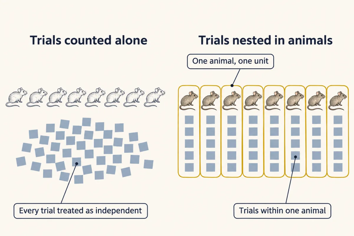
Chapter one used matched controls to identify an opsin-linked effect. When that effect looks large, how much evidence is enough? An experiment can record hundreds of responses without having hundreds of independent units. Repeated trials share each animal's expression, fibre placement and state. More trials sharpen that animal's mean. They do not create more animals. Eight mice each complete 40 trials. Does the study have 8 independent units, or 320?
In this design the independent unit is the animal. Keep its trials nested inside it during analysis. Treating every trial as independent erases shared variation within mice. The result then looks more precise than the experiment really is. For a two-group planning example, a standardized effect divides the difference between the means by the pooled spread. The same raw shift looks larger when outcomes cluster tightly. It looks smaller when the animals vary widely. Planning asks which effect is worth detecting, not which effect a small pilot happened to show. On a computed sample-size curve, smaller target effects demand much larger groups. The curve rises sharply because noisy overlap is harder to distinguish.
Small pilots give noisy effect estimates. The pilots that overshoot are also the most tempting to follow. If planning copies that lucky estimate, the confirmatory study can be too small before it begins. The same discipline applies to human imaging, where many brain-wide associations among people are small. A blood-oxygenation signal is not a spike count. A group average also does not guarantee stable rankings of individuals. Precision and reliability are different checks. A larger sample narrows uncertainty around an association.
Repeating the measurement asks whether people keep similar relative scores. A strong group average cannot substitute for either check when the goal is an individual biomarker. Keep three claims separate. Association says two measures vary together in a sample. Held-out prediction asks whether a model travels to new people. Causation asks what changes after the proposed cause is changed. Prediction alone does not supply that intervention. So size the study for the effect that matters, keep observations inside their independent units, and report uncertainty. Then match the final verb to the design. A precise association is still an association.
A controlled intervention can support a causal claim within its tested scope. Match the claim to the contrast and the sample.
From the film
- In this design, the animal—not each repeated trial—is the independent experimental unit.
- A standardized effect compares a group difference with the variability around it.
- Smaller effects require larger samples for the same power target.
- Association and held-out prediction do not by themselves establish causation.
Effect size, power and the experimental unit
The second film named the planning formula and kept trials inside animals; here is the arithmetic. The numbers below are invented for teaching.
Suppose a pilot gives a mean avoidance time of 60 seconds in the opsin-plus-light group and 48 seconds in the fluorophore-plus-light group, with a pooled standard deviation of 12 seconds. The standardized mean difference is the group difference divided by that pooled spread:
d = (60 s − 48 s) / 12 s = 1.0
For 80 percent power at a two-sided alpha of 0.05, the normal approximation for two independent groups is:
n per group = 2 (1.96 + 0.84)2 / d2
At d = 1.0, this gives 15.7, so the pilot implies 16 animals per group, or about 17 after allowing for a t distribution rather than a normal one. That is not automatically the planning answer. Small pilots estimate effects imprecisely, and the pilots that overshoot are more likely to be followed up. The effect carried into a confirmatory study therefore tends to be too large.
Plan for the smallest effect worth detecting. If that effect is d = 0.5, the same approximation gives 15.7 divided by 0.25, or 62.7: 63 animals per group.
- Fraction with p < 0.05: observed | expected
- —
- Mean observed d among followed-up pilots | expected | true d
- —
- Planning formula at this true d: n per group
- —
The lesson’s pilot: d = (60 s − 48 s) / 12 s = 1.0, so n per group = 2 (1.96 + 0.84)² / 1.0² = 15.7, which is 16 animals per group (about 17 with a t distribution). At d = 0.5 it is 15.7 / 0.25 = 62.8, so 63 per group.
Press Resample to draw 200 experiments.
In this sketch: normal data, equal and known SD (z test), two-sided α = 0.05, 80% power as the planning target, one number per animal, invented numbers. Expected fraction = Φ(d √(n/2) − 1.96) + Φ(−d √(n/2) − 1.96), derived from the lesson’s formula (the second term is the opposite tail). “Followed up” means significant with the opsin group higher. Eight mice with 40 trials each is n = 8, not 320. The lesson’s correlation arithmetic (n about 780 for r = 0.10) is left to the text.
Rule to keep: power the confirmatory study on the smallest effect you would care about, not on the pilot.
The film’s nested dots become an analysis choice. Reporting guidelines ask investigators to identify whether the independent experimental unit is an animal, litter or cage. Trial-level scoring is fine when the model preserves the nesting: repeated observations share expression, placement and state within an animal. Treating them as independent hides that shared variation and makes uncertainty too small, which is an easy route to a significant result that will not replicate.
Association, prediction and causation in human imaging
The second film separated association, held-out prediction and causation. The measurement and validation tests below decide which of those verbs a human imaging study has earned.
First ask what was measured. The conventional imaging signal indexes blood-oxygenation changes associated with neural activity, not spikes. In monkey visual cortex, Logothetis and colleagues recorded electrically and with that signal at the same time. Local field potentials estimated it better than multi-unit activity did, which led them to suggest that it reflects input and intracortical processing rather than spiking output. For recording many neurons directly, see recording many neurons.
Next ask how precise and stable the individual differences are. In Marek and colleagues’ rigorously denoised analysis of 3,928 ABCD participants, the median absolute univariate brain-wide association with behaviour was 0.01. The largest univariate correlation that replicated out of sample had an absolute value of 0.16. Replication improved as samples grew into the thousands, and independent subsamples of 25 could support opposite conclusions about the same association.
Elliott and colleagues pooled 90 task-fMRI experiments with 1,008 participants and reported a mean test-retest intraclass correlation of 0.397. A group-average activation can be clear while individual rankings are too unstable for a useful biomarker.
Keep the scope. These results concern brain-wide studies of individual differences. They do not say imaging is broken or set a minimum sample for every within-subject design, where each person is their own comparison. Marek and colleagues reported larger associations for functional than structural measures, cognitive tests than questionnaires, and multivariate than univariate methods. The univariate values above do not set a ceiling across designs. Sampling scheme, behavioural reliability and separating within-person change from between-person differences also change what can be detected at a given sample size.
Here is the precision calculation to run before trusting an association. Suppose the true correlation is 0.10, the order of magnitude Marek and colleagues report. With the Fisher transformation, atanh, the sample size for 80 percent power at a two-sided alpha of 0.05 is:
n = (2.80 / atanh r)2 + 3 = (2.80 / 0.1003)2 + 3 = about 780
Now take 25 people. The standard error on the transformed scale is 1 divided by the square root of n − 3, or 1 / sqrt(22) = 0.213.
Predict. An observed correlation is 0.10. Before calculating its interval, can this sample establish even the sign of the association?
Check your prediction
No. The 95 percent interval on the transformed scale is 0.100 ± 1.96 × 0.213, from −0.318 to +0.518. Converting back gives correlations from about −0.31 to +0.48. The sign is unknown. That is the arithmetic behind two subsamples of 25 disagreeing.
Held-out prediction adds a different test, but only if the outcome remains unseen. Feature selection and model tuning must happen inside the training data, and all scans from one person must stay in the same fold.
Predict. A model selects features using all participants, then cross-validates only the model fitting. Is its test performance genuinely held out?
Check your prediction
No. The test-fold outcomes already influenced feature selection, so the reported performance is optimistic. Repeat feature selection and model tuning inside each training fold.
Return to the rule: the claim cannot outrun the contrast. A validated predictor may generalize to new people while still leaving the cause of the predicted outcome unknown.
Design problem
A paper reports the following. Twenty patients and twenty controls are scanned. The authors search all connections and symptom measures, pick the strongest relationship, and report cross-validated prediction after splitting each person’s two scans across different folds. They name a mouse projection as the cause of the disorder, then activate that projection with light, comparing light-on with light-off in opsin-expressing animals, scoring avoidance unblinded, and counting each trial as a replicate. Their discussion proposes stimulating the human homologue as a treatment. Rewrite the study.
Saved in this browser only.
One way to do it
Start by separating three claims: an association in humans, a prediction target and a causal intervention in mice. A cross-sectional scan plus an acute mouse assay can suggest a mechanism, but it does not establish the mechanism of a human disorder.
On the human side, prespecify the imaging target or validate it in an independent sample. Do feature selection and model tuning inside the training folds. Split by person, so no participant appears in both training and evaluation. Report the effect size and uncertainty, not a p value alone, and measure test-retest reliability of the proposed marker. Forty participants cannot resolve an association of the size this literature reports, so join a large cohort or reframe the question as a within-person design. Check medication, head motion and recruitment as alternatives.
On the mouse side, add the opsin-negative arm and use the light-by-construct interaction, because light alone can change firing and behaviour. Verify expression, placement and physiology blind, including the period after illumination. Run activation for sufficiency and silencing for necessity in the same prespecified window. If the claim is projection-specific, test local transmission. Randomize allocation, blind scoring, define exclusions in advance, and analyze trials nested within animals.
Then write the conclusion the design supports: replicated, controlled evidence that activity in a named projection contributes to an assay-defined behaviour in mice during a defined window, alongside a separately reported human association with its uncertainty and reliability. A therapeutic claim would need human interventional evidence, which this study does not contain.
Going deeper
What the first channelrhodopsin experiments established
The tool has two separate histories. In 2003 Nagel, Bamberg and colleagues characterized channelrhodopsin-2 as a directly light-switched, cation-selective channel in Xenopus oocytes and mammalian cells. They also reported that continuous light desensitized it to a smaller steady-state conductance.
In 2005 Boyden, Zhang, Bamberg, Nagel and Deisseroth expressed that channel with a lentivirus in cultured rat hippocampal neurons and showed reliable millisecond-timescale control of spiking. The neurons came from newborn rats; there was no intact animal and no behaviour. Other groups expressed the channel in neurons around the same period, so there is no useful single “inventor” or “first” to award. The specific advance was control of spikes in chosen cells, which made a sufficiency experiment possible. The channel’s gating and selectivity belong to ion channels as receptors, and genetic targeting connects to CRISPR and functional genomics.
When the construct name misleads
Three failure modes deserve recordings rather than assumptions. Long channelrhodopsin-driven depolarization can suppress spikes through depolarization block, so driving harder can silence the cell meant to be driven. Anion-conducting silencers can excite compartments with high internal chloride, including some axonal compartments. Abruptly ending silencing can produce rebound firing, so the post-light window belongs in the result. Validate the physiology in the preparation during and after illumination.
Your notes
Select any text in the lesson to highlight it or add a note to it. Your highlights and notes are saved in this browser and collected in your notebook.
This browser is not letting the site save anything (a private window or strict privacy settings), so highlights and notes will be lost when you leave the page.
How we measure it
Optogenetic gain and loss of function
Express a light-sensitive channel or pump in genetically specified cells, then drive or suppress their activity at a chosen time while an animal behaves. Driving tests whether that activity is sufficient for the measured change; suppressing tests whether it is necessary. Each conclusion is scoped to those cells, that timing and that assay.
Whole-cell patch clamp
Record current and voltage from one neuron with a pipette sealed to its membrane. In an optogenetic experiment it is the validation step: it shows that light actually produced, or prevented, the spikes you assumed it did.
Task fMRI with test-retest reliability
Measure the blood-oxygenation signal while a person performs a task, and scan the same people twice to ask whether their individual scores are stable. An intraclass correlation summarizes that stability, and a group-average activation map does not substitute for it.
Held-out prediction and cross-validation
Fit a model on part of a dataset and evaluate it on observations not used in fitting. It estimates prediction, not causation, and it is only honest if feature selection happens inside the training data and the split is by person.
Practice questions on this lesson (3) → MCAT-style, original, each with an explanation
Where this lesson fits
Before thisReview first
- Emotion and StressThis course · Lesson 20
You need the amygdala structures from there to follow the basolateral-to-central amygdala projection experiment here.
- Recording Many Neurons: Imaging, Arrays and AtlasesThis course · Lesson 27
You need its account of what recordings and imaging measure to judge the imaging association claims here.
Suggested by an AI model from the lessons themselves, then checked. How we use AI
Finish line
Test yourself
8 questions
Practice and MCAT-style, with explained answers.
That's the last lesson · Next course
Physiology
How the human body’s organ systems work, measured: pressures, flows, volumes and the experiments behind them.
Start the next course →Before you move on: review the questions you missed , or go back to all lessons in this course.
← Lesson 27 · Recording Many Neurons: Imaging, Arrays and Atlases