Ecology and Evolution · Unit 4: Interactions and communities
Island Biogeography
Rewritten on : new text, flashcards and film. Your notes and highlights stay, but the text around them may have moved.
Empty an island of every insect and spider. How many species come back, and are they the same ones?
Pause when the reading reaches a film, and offer to play it. Saved on this device.
Watch the film now, or keep listening
Builds on:Population Growth and RegulationDistributions, Niches and TolerancesWhy these?
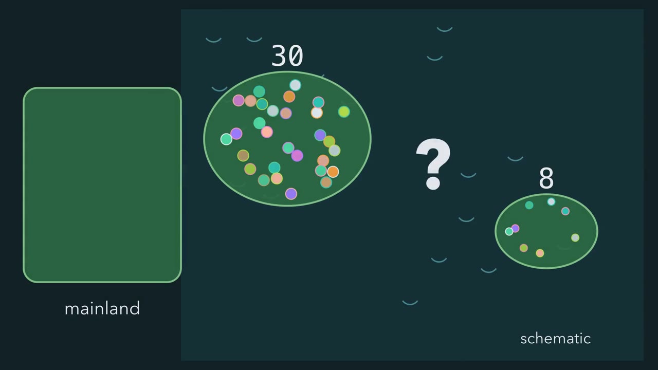 ▶ Watch Two Rates, One Crossing · 3:15
Read the transcript of “Two Rates, One Crossing”
Film transcript: Two Rates, One Crossing
Why does a big island near a mainland hold more kinds of animals than a small, remote one? One process can give both patterns. It is a balance between two rates. Start with the mainland. It holds a pool of species that could reach the island, P species in all. The number living on the island is S, its species richness. Now let animals cross the water. On an empty island, every arrival belongs to a new species, so the count climbs fast. Immigration, here, means only the arrival of a species not already present. As the island fills, more arrivals belong to species already there. An arrival of a kind already present changes nothing in the count.
So new arrivals slow, and stop when all P species live there. Plot that rate of new arrivals against the number of species on the island. The blue line starts high on an empty island and falls to zero when S reaches P. Residents also disappear. This is local extinction, a loss from this island only. Suppose each resident has the same, independent chance of being lost. Then more residents mean more losses, and the red line rises. Where the blue line meets the red, new arrivals equal losses. That richness is the equilibrium, S Below it, arrivals win and the count climbs. Above it, losses win and the count falls back. At the crossing, nothing stops.
Species keep arriving and keep vanishing, at the same rate. That shared rate is the turnover. The count settles near S star and wobbles a little, while the list keeps changing. Now push the island farther from the mainland, keeping its size the same. Which line moves, and which way does the gold point go?
Fewer new species reach a distant island at every richness. So the blue line drops, the crossing slides left, and S star falls. The far island holds fewer species. Now keep the distance and shrink the island instead. A small island loses residents faster at every richness. The red line rises, and S star moves left again. So near, large islands hold the most species, and far, small ones the fewest. One balance of two rates gives both of the old patterns. Keep the scope. This is a model. It leaves out new species forming on the island. Real curves need not be straight, because species differ and affect one another. And it predicts how many species, not which ones.
From the film
- An island's species count changes at the rate new species arrive minus the rate resident species are lost.
- Arrivals of new species slow as the island fills and losses speed up, so the count settles near where the two rates are equal.
- A farther island receives fewer new species and a smaller island loses species faster; both lower the equilibrium number, S*.
- At equilibrium species keep arriving and disappearing at the same rate, the turnover, so the count holds roughly steady while the list changes.
- This is a model: it leaves out new species forming on the island, real curves need not be straight, and it predicts how many species, not which ones.
The first film showed why near, large islands hold the most species, but not how fast an emptied island refills, or whether the returning species are the ones that left.
The one idea. An island’s species count changes at the rate new species arrive minus the rate resident species are lost. Arrivals of new species slow as the island fills and losses speed up, so the count settles near where the two rates are equal, while the species themselves keep being replaced.
Scope: one island fed by a mainland (or nearby islands), with new species forming on the island left out (Going deeper); this scope holds throughout. It is a model of rates: it predicts how many species and how fast they turn over, not which ones. Habitat fragments on land are only partly islands.
Two rates and a crossing
A cistern with a float valve works the same way: as the water rises, the float throttles the inflow and the drain runs faster, so the level settles while the water keeps changing.
In words The change in species number per unit time is the immigration rate of new species minus the local extinction rate. Both rates depend on how many species are already there.
- S“S”
- species now living on the island (richness)species
- P“P”
- the species pool: species that could reach the islandspecies
- I(S)“I of S”
- immigration: arrivals of species not already present, per unit timespecies per day
- E(S)“E of S”
- local extinction: residents lost from this island only, per unit timespecies per day
- S*“S star”
- the richness where the two rates are equalspecies
Sanity check On an empty island only immigration acts, so S rises. When all P pool species are present, immigration is zero and only extinction acts, so S falls.
In symbols, the film’s crossing S* is where dS/dt = 0. It is stable (nudge richness away and it returns), and the turnover is I(S*) = E(S*).
The count wobbles around S* because arrivals and losses are chance events. A smaller pool, which the film skipped, also lowers S*, since immigration reaches zero sooner.
Inset: richness S filling from an empty island (day 0)
- Equilibrium S* (I = E)
- Turnover at S*
- Richness reaches 90% of S*
- Net change at that richness
| Quantity | Expected | Simulated (this run) |
|---|---|---|
In this sketch: the curves assume continuous, deterministic change; the random run adds chance. Constant coefficients, no speciation, an empty island at day 0, pool P = 100 species; the numbers are invented teaching inputs, not estimates for any real island. In the random run each absent species arrives at the same rate I₀/100 per day and each resident goes extinct at rate e per day, independently.
Rule to keep: richness settles where immigration equals extinction, and at that point species are still arriving and leaving at the turnover rate.
Working the numbers
Worked problem. The numbers are invented, not estimates for any real island. An island draws on a pool of P = 100 species. Immigration is I(S) = 10(1 - S/100) species per day and extinction is E(S) = 0.1S species per day: extinction is proportional to S, as when each resident has the same independent chance of loss. Assume continuous, deterministic change (no chance events), constant coefficients, no speciation, and an empty island at time zero.
- Equilibrium. dS/dt = 10 - 0.1S - 0.1S = 10 - 0.2S. Setting this to zero gives S = 50 species*.
- Turnover. At S = 50, I = 10 x 0.5 = 5 species per day and E = 0.1 x 50 = 5 species per day. Net change is zero, yet about 5 species are replaced each day (10 events per day if you count gains and losses separately).
- Approach (calculus; optional). The 0.2 per day in step 1 is a continuous rate constant (0.1 from slowing arrivals plus 0.1 from faster losses), so the gap to S* decays exponentially, shrinking about 18% each full day (e−0.2 = 0.82). Solving from S = 0 gives S(t) = 50(1 - e−0.2t). Richness reaches 90% of S*, 45 species, when e−0.2t = 0.1, so t = ln 10 / 0.2 = 11.5 days. Check: at S = 45, I = 5.5 and E = 4.5 species per day, so richness is still rising by 1 species per day.
Predict. A smaller island has a lower S*. Does it also turn over more slowly, or faster?
Check your prediction
Faster, in the model. A smaller island is a steeper red line: double the extinction coefficient from 0.1 to 0.2. That lowers S* to about 33, but about 6.7 species are then replaced each day, against 5: fewer residents, each lost more often. Nearness, by contrast, raises both S* and turnover.
| Island (one change from steps 1 and 2) | S* | Turnover per day |
|---|---|---|
| Original | 50 | 5.0 |
| Nearer: I(0) = 15 | 60 | 6.0 |
| Farther: I(0) = 5 | 33 | 3.3 |
| Smaller: E = 0.2S | 33 | 6.7 |
| Larger: E = 0.05S | 67 | 3.3 |
The table’s pattern is the model’s, not a measured one: real species differ in extinction chances and change one another’s chances, so real curves need not be straight.
The worked island, started empty, reaches about 47 species, 94% of S*, within two weeks, though the count says nothing about which species. The rare real islands that are refilling, such as Krakatau, cannot be replicated or controlled, so the second film’s islands were emptied on purpose.
Read the transcript of “Emptying Islands”
Film transcript: Emptying Islands
The worked island refilled on paper, toward a steady count, while species kept coming and going. So empty a real island of every insect and spider. How many species come back, and are they the same ones? Most islands were colonised long ago, so nobody saw their rates from the start.
Daniel Simberloff and Edward Wilson chose islands small enough to empty, and then watched them fill. They used six small islands of red mangrove in the Florida Keys. Each carried a community of terrestrial arthropods: insects, spiders, mites and their relatives. First they recorded every arthropod species on each island. Then they covered each island with a tent and fumigated it. Afterwards they censused the islands again and again for a year. The count climbed back. By about day 250, most islands held about as many species as untreated islands. The exception was E1, the most distant.
Population densities, though, were still abnormally low. Now the second question. The count came back. How much of the old species list do you expect the new list to share? Take three mite kinds from island E9, chosen because their records are clear. One was there before and after. One was there only before. One was there only after. Two kinds before, and two kinds after, so the count is unchanged. But only one of the three is shared. The Jaccard similarity is shared species divided by species in either list. Here it is 1/3. Read it with care. These three are a chosen subset, not the whole community. And finding the shared mite at both censuses does not mean it survived.
It was recorded again after recolonisation. A second report followed four islands to the end of the second year. Species numbers had changed little from the year before, while immigrations and extinctions continued at high rates. A steady count with continuing replacement is what the model calls a dynamic equilibrium. The result fits the model, though on its own it does not prove the model's mechanism. And the rates themselves were rough. Censuses came at intervals, so some arrivals and losses fell between visits and were never seen. And a resident overlooked at one census looked like a loss and a return.
From the film
- Simberloff and Wilson censused the arthropods on six small red mangrove islands in the Florida Keys, removed them by fumigation under a tent, and censused again for a year.
- By about day 250, all but the most distant island, E1, held species numbers similar to untreated islands, though population densities were still abnormally low.
- The returning species were not all the ones present before, and in the second year arrivals and losses continued while the count changed little.
- The Jaccard similarity, species shared divided by species in either list, separates which species are present from how many.
- A steady count with a changed list fits a dynamic equilibrium without proving its mechanism, and census gaps make the measured rates rough.
Testing it: emptying islands in the Florida Keys
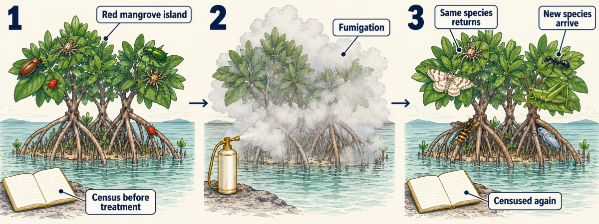
How they came and went. The authors inferred that most arrivals came through the air, by flight or carried on the wind. They also considered physical causes important in the extinctions of early colonists, so not every loss can be read as one species excluding another.
Area by itself. Large islands also differ in habitat, so in a 1976 study Simberloff censused eight mangrove islands, removed sections to reduce their area, and censused them again. Richness tracked island area independently of habitat diversity in that system, though the sample was too small to test whether smaller islands also turn over faster, as the table above predicts.
Same number, different species
The second film’s three E9 mites shared one third of their list, and it was not just those three: in the 1969 report, the species on each island were not all the ones present before treatment. A caution the film did not give: dividing the mites’ changes by 364 days does not give a turnover rate, because other arrivals and losses between censuses are not counted. Is one third low for an island at equilibrium?
Predict. Make the worked island a chance process in which every species comes and goes independently of the others: each absent pool species arrives at a rate of 0.1 per day, and each resident is lost at a rate of 0.1 per day (continuous rates, as in step 3, not daily chances), every species alike. Census it at equilibrium, then 5, 10 and 100 days later. Does the shared fraction keep falling toward zero?
Check your prediction
No. With equal rates in and out, each species is present half the time, and because species act independently, S wobbles around 50 (standard deviation about 5); species that came and went together would make the count swing far more. The expected Jaccard similarity falls from 1 to about 0.52 after 5 days and 0.40 after 10, then levels off near 0.33. It stops at a third because, long after, each species’ presence at the two censuses is like two independent coin flips: on both lists with chance 1/4, on neither with chance 1/4, so on at least one with chance 3/4, and 1/4 ÷ 3/4 = 1/3. With every species alike, a steady count sharing a third of its list is what this model expects; species present more or less than half the time give other values. The E9 three are hand-picked, so their one third is only a scale check.
For comparing communities by identity, see diversity and succession.
Fragments, area and connectivity on land
A forest remnant surrounded by farmland looks like an island, and the species-area pattern is often summarised as S = cAz, where A is area and the fitted constants c and z set the overall level and how fast richness rises with area. The exponent z varies among taxa (groups of organisms) and sets of islands, so treat any single value as illustrative.
Worked problem, continued. Take z = 0.25.
- Habitat loss. A habitat holding 50 species is cut from 100 to 10 km2. Richness is multiplied by (10/100)0.25 = 0.56, so it falls toward about 50 x 0.56 = 28 species. If the same curve holds for the remnant, this is the long-run value after relaxation, the slow loss of species that a smaller area can no longer hold, not a loss on the day of the cut. Treat it as a rough projection: some species survive in the surrounding land, and the method itself is debated (Going deeper).
Fragments are not true islands: the surrounding land, the matrix, is not open sea. Some species live in it, some cross it readily and some cannot cross it at all. That ties the model to the metapopulation view: a set of local populations linked by dispersal, each subject to local extinction and recolonisation.
Rates can be a more sensitive signal than counts. In Swiss Jura grassland patches that Jasmin Joshi and colleagues isolated by mowing from 1993 to 1999, plant colonisation was 30% lower than in unisolated controls, yet after seven years the patches had only marginally fewer species, perhaps because counts lag behind rates, as in relaxation.
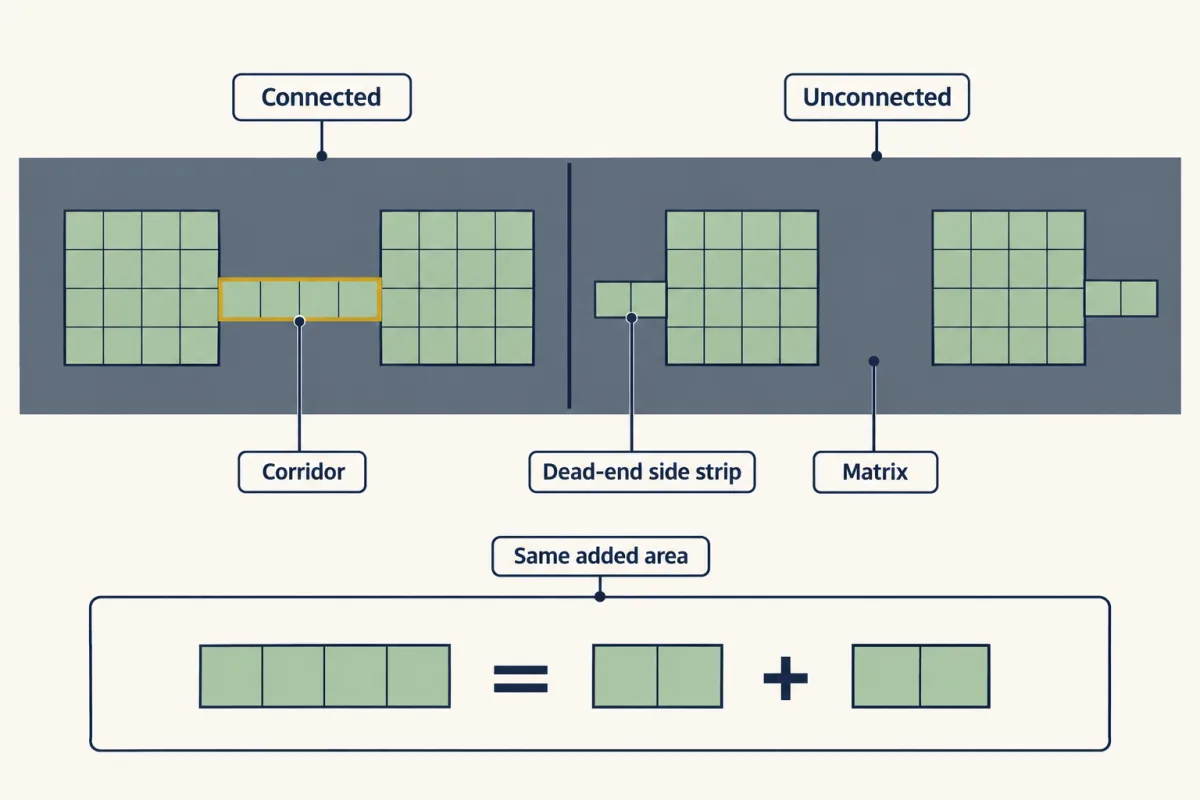
Connectivity has been tested over a longer span. In a longleaf pine savanna experiment reported by Ellen Damschen and colleagues (Science, 2019), patches joined by corridors had annual colonisation about 5% higher and annual extinction about 2% lower than unconnected patches across 239 plant species. After almost two decades, connected patches held nearly 14% more species and were still gaining; a five-year study would have seen much less of the effect. For reserve planning, see conservation.
Design problem
A planner must choose between one 100 ha reserve and four 25 ha reserves, or decide whether to link existing patches with corridors. Design a study that tests whether connection itself changes the species found in patches.
Saved in this browser only.
One way to do it
Island biogeography alone does not settle the reserve choice: one large reserve may hold more area-sensitive species, while several small ones may sample more habitat types and spread the risk of a local disaster. So test the mechanism.
- Replicate equal-area patches in the same kind of habitat and matrix, and assign them at random to connected or unconnected treatments.
- Control for the corridor’s own area. A corridor adds habitat and edge. Give some unconnected patches dead-end side strips matching the corridor’s area and edge-to-area ratio, and others the same extra area as a plain block, so a difference can be attributed to connection.
- Census species identity repeatedly, at a fixed effort and season, for many years, recording which species are present as well as how many.
- Estimate colonisation and local extinction separately, from changes in each species’ presence between censuses, and say how many events between visits you could have missed.
- Report both richness and composition (for example Jaccard similarity to a reference patch). Effects can keep growing for years, although in the same system the effect on bird-dispersed plants had levelled off.
The result applies to that habitat, matrix and set of species; whether it transfers to another matrix or to animals with other dispersal modes needs its own test.
Going deeper
Speciation and the book
MacArthur and Wilson also counted speciation on the island as a further source of species, which matters on large, remote islands, not small mangrove ones. Where it is appreciable, its rate adds to immigration, and the count settles where immigration plus speciation equals extinction. Their 1967 book, The Theory of Island Biogeography, developed the theory at length.
The defaunation method
The islands were red mangrove, Rhizophora mangle, and each was tented and fumigated with methyl bromide; the full one-year report appeared in Ecology in 1969, and a second report in 1970 followed four islands to the end of the second year (the steady count the second film ends on). The 1969 appendix marks each record as seen, inferred present or inferred absent; the film’s E9 mites were chosen for unambiguous records. Treatment had its own side effects: on island E7, fumigation killed 85% of the mangrove tree.
How rough the measured rates were
Most observed immigration and extinction rates lay between 0.05 and 0.50 species per day, against about 0.1 to 1.0 from a simple noninteractive model (species do not change one another’s chances). The authors suggested many events between censuses went unrecorded.
Running a species-area curve backwards
Step 4 used a species-area curve in reverse, predicting losses from a shrinking area. Whether that overestimates extinctions after habitat loss is debated.
Your notes
Select any text in the lesson to highlight it or add a note to it. Your highlights and notes are saved in this browser and collected in your notebook.
This browser is not letting the site save anything (a private window or strict privacy settings), so highlights and notes will be lost when you leave the page.
How we measure it
Experimental defaunation and repeated census
Every species on a small island is recorded, the fauna is removed (here by methyl bromide fumigation), and the island is censused again at intervals. Comparing species lists between censuses gives colonisations and local extinctions, though events that begin and end between visits are missed.
Experimental area reduction
Parts of an island are removed and the remaining fauna is recensused. Because the same island is compared before and after, area changes while habitat type and location stay much the same, which a comparison across different islands cannot achieve.
Replicated connectivity experiment
Equal habitat patches are created and assigned to connected or unconnected treatments, with controls for the area a corridor adds. Colonisation and extinction are estimated separately from repeated surveys of species identity over many years.
Presence-absence comparison (Jaccard similarity)
Two species lists are compared by dividing the number of species they share by the number found in either. Equal richness can hide a low similarity, so the index separates how many species are present from which species they are.
Practice questions on this lesson (3) → MCAT-style, original, each with an explanation
Where this lesson fits
Before thisReview first
- Population Growth and RegulationThis course · Lesson 14
You need rates of gain and loss setting a population's size, and the logistic balance point, before applying them to species counts.
- Distributions, Niches and TolerancesThis course · Lesson 12
You need to know why species occur where they do and fail to reach other places before reading immigration rates.
After thisStudy next
- Conservation and RestorationThis course · Lesson 25
This lesson sends you there to apply area, isolation and corridor results to reserve design.
- Global Change: Species on the MoveThis course · Lesson 24
Shrinking habitat and range shifts use the same arrival-and-loss rates to judge which species persist.
Elsewhere on the siteFilms, simulations and method films in other courses
- Occupancy modelling and eDNA surveysMethod film
Island censuses miss species, and this method shows how to judge presence when detection is imperfect.
Suggested by an AI model from the lessons themselves, then checked. How we use AI
Finish line
Test yourself
8 questions
Practice and MCAT-style, with explained answers.
Next · Lesson 21
Energy Flow and Productivity
In a made-up budget, plants on one square metre fix 12,000 kilojoules a year and the top predators make 40. Where did the rest go?
Continue →