Ecology and Evolution · Unit 6: Global change and decisions
Integrative Evidence Workshop
Rewritten on : new text, flashcards and film. Your notes and highlights stay, but the text around them may have moved.
Twenty negative PCR wells from one pond. Is the newt gone?
Pause when the reading reaches a film, and offer to play it. Saved on this device.
Watch the film now, or keep listening
Builds on:Movement and Spatial PopulationsConservation and RestorationGlobal Change: Species on the MoveWhy these?
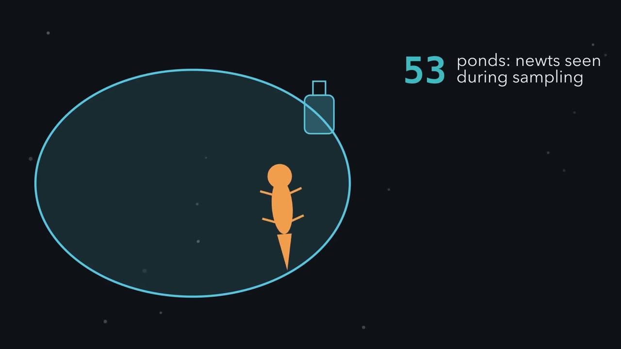 ▶ Watch What a Negative Is Worth · 3:28
Read the transcript of “What a Negative Is Worth”
Film transcript: What a Negative Is Worth
When every test from a pond comes back negative, what have you learned? Is the species gone? At 53 English ponds, newts were seen while the water was being sampled. Yet 13% % of those samples, about seven, showed no newt DNA.
A survey is a series of nets with holes. First, DNA must be in the water you scoop. That chance is theta. Second, the extraction must capture it. That chance is gamma. Third, one qPCR well must amplify it. That chance is delta. Together, the nets give one number, q. It is the chance that one water sample detects a pond that really is occupied. Here we use a round number: q is one half. Now picture a hundred ponds like yours. Before sampling, we think twenty of them hold the species. Those are teal. The other eighty, in grey, are empty. With no false positives, an empty pond always tests negative. Sample every pond once. Half the occupied ponds light up as detections and leave the pile.
Ten occupied ponds stay hidden among eighty empty ones. The share of negative ponds still occupied drops to eleven percent. Now take a second, independent sample from every pond that is still negative. How many hidden occupied ponds will remain? And what share of the negative ponds will still hold the species?
Half of the ten hidden ponds are caught. Five stay hidden, among 85 negative ponds. The share falls to about 6%. percent. A third sample leaves 2.5 hidden ponds on average, about 3%. percent. The side bar tracks the chance that a negative pond is still occupied. It falls with every independent sample, but never reaches zero.
The grid is the equation. On top sit the hidden occupied ponds: the prior, times the chance an occupied pond misses every time. Below sit all the negative ponds: the empty ones, plus those hidden ones. Two numbers here are set by us, not measured by this survey. One is the prior, how likely occupancy was before sampling. The other is the stop line, here five percent. Change either, and the samples you need change. The count also assumes no false positives. Each pond stays occupied or empty for the whole survey. And each sample is an independent try. So a negative never proves absence. Each negative sample multiplies the hidden ponds by the miss chance.
The empty ponds stay put. But is every test you run a new try?
From the film
- A negative eDNA result does not show that a species is absent: DNA can be missed in the water, in the extraction or in the qPCR well.
- Together, the three steps set q, the chance that one water sample detects an occupied pond: its water must hold DNA, and at least one extraction must capture it and have a well amplify it.
- Each independent negative sample multiplies the occupied sites still hidden among the negatives by that miss chance, while the empty sites stay put, so the probability of occupancy falls with every new sample but, as long as a sample can sometimes detect and sometimes miss, never reaches zero.
- That probability is the hidden occupied sites divided by all the sites that tested negative, so it also depends on how likely occupancy was before sampling (the prior).
- The count assumes no false positives and a site that stays occupied or empty for the whole survey.
The first film counted ponds with round numbers. Here we run it on data, decide, test how firm the decision is, and ask who decides how data are used. Background: spatial populations, conservation and global change.
The one idea. A run of negatives never proves a species is absent. Each independent negative water sample multiplies the occupied ponds still hiding among the negatives by the chance that an occupied pond is missed, while the empty ponds stay put. So the share still occupied falls with every sample but never reaches zero. (This needs a prior between 0 and 1 and a sample that can both detect and miss.) Wells and extractions from one water sample all test that sample’s water, so they cannot lift its detection above the chance the water holds DNA. Only new water is a new try at the scoop.
What eDNA detects and what it misses
Environmental DNA (eDNA) is DNA collected from an environmental sample, such as water, soil or air, rather than from the organism itself; for animals, much of it is DNA they shed. A targeted survey filters water, extracts DNA and runs a quantitative PCR (qPCR) assay for one species (recombinant DNA and PCR, sequencing and genomes). Each qPCR run, in one well of a plate, either amplifies the target or does not.
A site is occupied if the species uses it during the survey. A false negative is a miss: the organism or its DNA is present and nothing amplifies. A false positive is a report of the target when it is absent; contamination and a poorly specific assay are two routes.
The first film’s three nets get symbols, in its colours: θ (theta, blue), the chance that a water sample from an occupied pond holds the species’ DNA in a form the assay can detect; γ (gamma, green), the chance that an extraction captures DNA that is in the sample; and δ (delta, gold), the chance that one qPCR run amplifies captured DNA. One reason θ is below 1 is decay: it can leave too few intact copies of the target sequence in the scoop, even when shorter fragments remain. In upland Welsh stream mesocosms (outdoor experimental stream channels), DNA from three species fell by more than 90% within three hours and was nondetectable within two days, faster in acidic water (Seymour and colleagues, 2018): one experimental system, not a universal eDNA lifetime.
Detection probability and an all-negative site
Made-up great crested newt data: four ponds, two water samples each, two extractions per sample, five qPCR runs per extraction. Each string is one extraction’s five runs; 1 means amplification.
| Pond | Sample 1 (extraction 1 / 2) | Sample 2 (extraction 1 / 2) | Positive wells (of 20) |
|---|---|---|---|
| S1 | 10000 / 00000 | 00000 / 00000 | 1 |
| S2 | 00000 / 00000 | 00000 / 00000 | 0 |
| S3 | 00000 / 00000 | 00000 / 00000 | 0 |
| S4 | 11100 / 00000 | 11000 / 00000 | 5 |
Two of four ponds amplified at least once, so the naive occupancy estimate is 2/4 = 0.50. It ignores misses: S2 or S3 may be occupied. S1 counts as occupied only under the no-false-positive assumption below; its lone positive well is taken up after the decision.
Worked problem: is S2 still occupied? S2 gave 20 negative wells: 2 samples × 2 extractions × 5 wells.
| Measured elsewhere (borrowed, illustrative) | Our inputs |
|---|---|
| γ = 0.49, estimated without inhibitor removal | θ = 0.60 (assumed) |
| δ = 0.38 | prior = 0.20: our belief, before sampling, that S2 is occupied |
| Wild pigs, central Texas, one autumn (Amy Davis and colleagues, 2018); each has a standard error | Stop rule (a decision choice): stop when P(occupied) is 5% or below |
Assume no false positives (an empty pond always tests negative), S2 occupied or empty for the whole survey, and independence at every level: at an occupied pond, one sample missing does not change the chance the next one misses, and likewise for extractions from one sample and wells from one extraction. θ and the prior are assumed; a real analysis would estimate or inform them from relevant data, but four ponds are far too few to do so reliably. Work from the inside out with the product rule from probability and crosses: replicates at one level all miss with the product of their miss chances, and detection needs every step to succeed.
- Wells. One run misses with 1 − 0.38 = 0.62; all five miss with 0.625 = 0.092. So five wells catch captured DNA with A = 0.908.
- Extractions. One extraction finds the DNA only if it captures it and the wells catch it: 0.49 × 0.908 = 0.445, so it misses with 1 − 0.445 = 0.555. Both miss with 0.555² = 0.308, so the pair finds DNA in the water with B = 0.692.
A sample detects only if its water holds DNA and the lab finds it, so q, the first film’s chance that one water sample detects an occupied pond, is θ × B.
Predict. The water holds DNA only 60% of the time. Will q be closer to 0.69 or to 0.40?
Check your prediction
- Sample. q = 0.60 × 0.692 = 0.415, closer to 0.40: the scoop sets the ceiling.
- Two samples. Each sample misses with 1 − 0.415 = 0.585, so two independent samples both miss an occupied pond with m = 0.585² = 0.342.
- Weigh against the prior. Count as the first film did: of 100 ponds like S2, 20 are occupied and 20 × 0.342 = 6.8 of them stay hidden among 6.8 + 80 = 86.8 all-negative ponds. That share is the posterior (the probability after the data):
P(occupied | all negative) = prior × m / [(1 − prior) + prior × m] = 0.068 / 0.868 = 7.9%
Predict. Stop, or sample again? If again, how many more negative samples will it take?
Check your prediction
- Decide. 7.9% is above 5%, so sample again. A third negative sample gives m = 0.585³ = 0.200 and 0.040 / 0.840 = 4.8%, just under the line.
- Chance all samples miss an occupied pond
- 0.342
- Chance an all-negative pond is occupied
- 7.9%
- Lowest possible with perfect lab work
- 9.1%
- Assumed rule: stop only at 5% or below
- Sample again
In this sketch: gamma = 0.49, delta = 0.38 and theta = 0.60 are illustrative values, there are no false positives, occupancy is fixed during sampling the stages are independent, and the 5% rule, theta = 0.60 and the prior are choices.
Extra qPCR wells share one sample, so they cannot push detection above theta; only another independent water sample attacks the missing share.
A third sample means another field trip. Why not run more wells instead?
Read the transcript of “Wells Share One Scoop”
Film transcript: Wells Share One Scoop
More wells cost an afternoon in the lab, not a field trip. Pond S2 already gave twenty negative wells. Are those twenty tries, or only two? Draw S2 as a tree. The pond gives two blue water bottles. Each bottle gives two green extraction tubes. Each tube feeds five gold wells. So all twenty wells hang from just two scoops of water. Use the workshop's numbers. A scoop holds DNA 60% % of the time. That is theta, the blue line. The capture and well values are borrowed from a wild pig study in Texas, as illustrations only. Try adding wells. Pour more gold wells under the same two bottles. The gauge for one sample climbs at first. Then it levels off, still below the blue line.
It never crosses theta, however many wells you add. The reason is simple. If the scoop held no DNA, every tube and every well from it is testing empty water. No number of wells can find DNA that the sample does not contain. Watch the bar for the chance that S2 is still occupied. With unlimited wells on two samples, it stops at 7.2%. That is still above the 5% percent line. Now add a third blue bottle instead, a new scoop of water from the pond. With the usual five wells per extraction, the bar drops to 4.8%. That is below the line. Here is a tempting mistake.
Suppose we pretend the twenty wells were twenty separate trips to the pond. Will the pond look emptier, or fuller, than the evidence allows? Emptier. Redraw the tree as twenty bottles, each with one well. Each one now looks like its own try. The bar plunges to about two percent, and you would stop. But you would stop on an error in the model, not on evidence. Counting repeated measurements of one unit as if they were separate units has a name. It is called pseudoreplication. So wells and extractions from one sample all test the same water. They are second chances at the lab steps, not new tries at the scoop. Here, adding wells cannot cross the line.
A third water sample does.
From the film
- Wells and extractions from one water sample all test that sample's water: they are second chances at the lab steps, not new tries at the scoop, so they cannot detect DNA the sample does not contain.
- However many wells you add, one sample's chance of detecting an occupied pond cannot exceed θ (theta), the chance the water holds DNA.
- In this example, adding wells to two samples (two extractions each) leaves an all-negative pond above the 5% line; a third independent water sample brings it below.
- Counting wells as if they were separate field samples is pseudoreplication: it makes a pond look emptier than the evidence shows.
Sampling design: field replicates versus PCR replicates
The second film called the twenty-well shortcut pseudoreplication (counting repeated measurements of one unit as separate units). It left out two things. First, the ceiling is on one sample, not on the decision: with enough extractions, even two samples can cross the line (Going deeper). And how firm is 4.8%? Davis’s γ has a standard error (SE, a measure of an estimate’s uncertainty) of 0.07.
Predict. Lower γ by one SE, to 0.42. After three negative samples, stop or continue?
Check your prediction
Continue: three samples now give 5.9%.
| P(occupied | all negative) | 2 samples | 3 samples | 4 samples |
|---|---|---|---|
| γ = 0.42 (one SE lower) | 9.0% | 5.9% | 3.8% |
| γ = 0.49 (worked problem) | 7.9% | 4.8% | 2.8% |
| γ = 0.56 (one SE higher) | 6.9% | 3.9% | 2.2% |
| γ = 0.49, unlimited wells | 7.2% | 4.1% | 2.3% |
New water samples move the posterior; unlimited wells barely do. Lowering γ by one standard error puts the third sample above 5%.
Our choices matter too: across θ from 0.5 to 0.7 and priors from 0.1 to 0.3, the negative samples needed run from 2 to 5. Report a decision this close to its line with its sensitivity.
In the English newt surveys analysed by Andrew Buxton and colleagues (2021), twenty subsamples from around each pond were pooled into one water sample: wider coverage, but one field sample, leaving no field replicates to estimate θ. In the Texas pig trial, the authors suspected that pooling each site’s ten samples diluted the DNA, and pooled data underestimated occupancy at sites known to be occupied. Buxton’s simulations found that replicating both field and lab work reduced bias and narrowed credible intervals (Bayesian ranges of plausible values). Only new water is a new try at the scoop.
What a positive can and cannot mean
So far we assumed no false positives. Clean blanks make contamination less likely but cannot exclude a rare, one-off event. S1’s single positive well out of twenty is the sparse pattern Buxton and colleagues judged more likely than others to be a false positive, and their two published models, one of which ignored false positives, gave overall occupancy of 0.26 and 0.47 for the same 2,958 English ponds surveyed in 2019 (one pooled sample each, twelve qPCR replicates). With no ground truth, the authors judged that the model ignoring false positives overestimated; false-positive parameters can need calibration or informative priors to be identified.
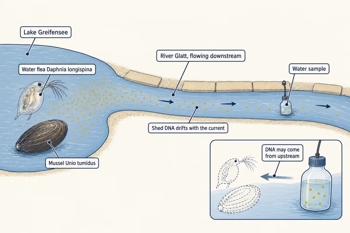
Place matters too: in flowing water, a true DNA detection can falsely signal occupancy at that spot. In the river Glatt below Lake Greifensee, Switzerland, Kristy Deiner and Florian Altermatt (2014) detected the lake-dwelling water flea Daphnia longispina at every sampled river location, as far as 12.3 km downstream, but did not detect the mussel Unio tumidus beyond 9.1 km.
Design problem
A river survey detects an endangered mussel’s eDNA at one site 5 km below a lake where the mussel lives. Does the mussel occur at the site? Design the follow-up.
Saved in this browser only.
One way to do it
A positive can mean a local population, DNA carried down from the lake, or contamination. In the Glatt, mussel DNA was detected downstream though not beyond 9.1 km, so transport over 5 km is plausible in at least one river.
- Check for contamination. Carry field blanks, extraction blanks and PCR negatives through every batch, and sequence positives to confirm the species.
- Test transport. Sample from the lake outlet down past the site, plus each tributary between. A local population would tend to add signal at and below the site; transport alone would tend to fade with distance from the lake. DNA settling on the streambed and stirred back up, and patchy flow, blur both patterns, so use replicate samples and flow data.
- Replicate in the field. Independent water samples on separate dates, not more wells; record flow and pH.
- Model and confirm. DNA carried from the lake is a false positive for this site, so the no-false-positive model above fits only once transport is excluded; otherwise use a model that allows transport or other false positives, with stated assumptions. Either way, search the site directly with a method suited to mussels.
- Agree access first. Settle with whoever governs the river and the data how results will be shared.
Reproducible analysis and the decision
Keep the raw file untouched; work on copies. A data dictionary defines every column: site, date, sample, extraction, PCR replicate, control, treatment, covariates. Record a non-detection differently from a missing, inhibited or inconclusive run; an inhibited well, where substances carried over from the sample blocked the PCR, is not a negative.
Sandve and colleagues (2013) set out rules that apply here: replace manual editing with scripts, archive the exact program versions, record every parameter and input, and record random seeds whenever an analysis uses randomness. FAIR (findable, accessible, interoperable, reusable) adds provenance and a clear licence. Then rerun from the raw file and check you get 7.9% and 4.8% again, with θ, the prior and the threshold beside them.
Whose data? CARE and FAIR
Surveys happen on someone’s land and water. FAIR makes data usable by machines and people, and it permits authentication and authorization; it does not mean open to all. The CARE principles for Indigenous data governance, drafted in Gaborone, Botswana, on 8 November 2018 and published in 2020, add the question of who decides: Collective Benefit (data should benefit Indigenous Peoples), Authority to Control (Indigenous Peoples determine governance protocols for their data), Responsibility (respectful relationships with the people the data come from) and Ethics (their rights and wellbeing are central across the data’s life). A 2021 paper describes CARE as a complement to FAIR that covers scientific data as well as traditional knowledge.
For eDNA, a rare species’ location in a community’s water is itself data whose release that community may have the authority to control. This workshop uses no real community dataset and claims no permission. Merging eDNA results with a community’s observations would first mean identifying the rights holders, the benefit and the permitted purpose, and getting their protocols; a downloadable file is not permission.
Going deeper
The model in one line
With w wells per extraction and k extractions per sample, A = 1 − (1 − δ)w and q = θ × [1 − (1 − γA)k]; n independent samples miss an occupied site with m = (1 − q)n. In odds, each negative sample multiplies the odds of occupancy by 1 − q: the hidden-pond count in other words. These equations assume no false positives, closure (occupancy fixed during sampling), conditional independence at every replicate level (wells, extractions and samples, as in the worked problem), and parameters constant across sites and visits (or explained by covariates). A model that allows false positives needs extra false-positive parameters, which must be identifiable, and a different posterior.
When lab work could cross the line
Perfect lab work makes q = θ = 0.60: one negative sample leaves 0.20 × 0.40 / (0.80 + 0.08) = 9.1%, two leave 3.8%. With unlimited wells an extraction still captures only with γ = 0.49, so q = 0.60 × [1 − 0.51k] for k extractions: two samples with four extractions each give 4.6% (three extractions, 5.4%).
The pseudoreplication arithmetic
Treating each of S2’s 20 wells as an independent try detecting with 0.60 × 0.49 × 0.38 = 0.112 gives a miss probability of 0.88820 = 0.094 and the second film’s 2.3%.
Carrying the uncertainty through
Borrowed point estimates hide their uncertainty and covariates (Davis and colleagues found DNA availability varied with month, pH and water-body type). The γ table is a one-at-a-time sensitivity check. For management use, compute the posterior across the joint uncertainty of γ, δ, θ and the other fitted parameters, with relevant covariates, and test whether the decision changes.
Your notes
Select any text in the lesson to highlight it or add a note to it. Your highlights and notes are saved in this browser and collected in your notebook.
This browser is not letting the site save anything (a private window or strict privacy settings), so highlights and notes will be lost when you leave the page.
How we measure it
Environmental DNA sampling with qPCR
Water is collected, filtered or precipitated, and DNA is extracted; a species-specific qPCR assay is then run several times per extraction. A run either amplifies or does not, and the pattern of runs, extractions and samples is the raw evidence of whether the species' DNA was there.
Multiscale occupancy modelling
A statistical model that treats occupancy as a hidden state and estimates, from the pattern of replicates, the probability of detection at each nested stage (DNA in the sample, captured in an extraction, amplified in a run). It turns a set of negatives into a probability that the site is still occupied.
Independent validation of occupancy
Cameras, field signs or direct surveys establish which sites are occupied by another route, so detection probabilities can be estimated at sites whose true state is known, as in the wild pig trial in central Texas.
Negative controls and sequence confirmation
Field blanks, extraction blanks and PCR no-template controls are carried through the workflow to flag contamination (blanks can reveal contamination that reaches them or runs broadly through a batch, but clean blanks cannot exclude localized or rare one-off contamination), and amplified products are sequenced to confirm that the signal comes from the target species and not a relative or an off-target product.
Practice questions on this lesson (3) → MCAT-style, original, each with an explanation
Where this lesson fits
Before thisReview first
- Movement and Spatial PopulationsThis course · Lesson 15
It explains that a patch can be occupied or empty and that occupancy changes over time, the idea the occupancy count builds on.
- Conservation and RestorationThis course · Lesson 25
It sets up why deciding whether a rare species is still present matters for management decisions.
- Global Change: Species on the MoveThis course · Lesson 24
The detection question here is posed for species whose ranges shift, which is where this lesson's background starts.
Elsewhere on the siteFilms, simulations and method films in other courses
- Pedigree analysisMethod film
It shows the same Bayesian step of turning a prior and a negative result into a probability of carrying or being present.
- Experimental units, pseudoreplication and powerMethod film
It teaches why replicates from one sample are not independent units, the pseudoreplication point of this workshop.
Suggested by an AI model from the lessons themselves, then checked. How we use AI
Finish line
Test yourself
8 questions
Practice and MCAT-style, with explained answers.
That's the last lesson · Next course
Biochemistry
The one-semester sequence: molecules, enzymes, membranes, metabolism.
Start the next course →Before you move on: review the questions you missed , or go back to all lessons in this course.