Cell Biology · Unit 5: Cells in tissues
New to this? Review it at high school level: One Cell or Many
Cell Identity, Cell State and Disease
Rewritten on : new text, flashcards and film. Your notes and highlights stay, but the text around them may have moved.
Much of the lining of an older person's healthy oesophagus can carry mutations found in cancer. Why is it still healthy?
Pause when the reading reaches a film, and offer to play it. Saved on this device.
Watch the film now, or keep listening
Builds on:Stem Cells and Tissue RenewalCyclin-CDK Control of the Cell CycleExperiments That Distinguish MechanismsWhy these?
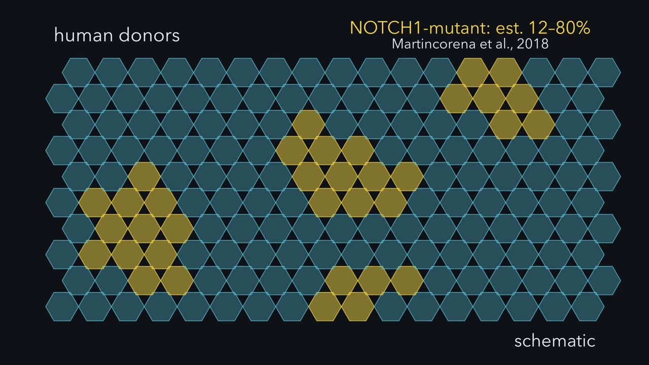 ▶ Watch Fate, Not Speed · 3:03
Read the transcript of “Fate, Not Speed”
Film transcript: Fate, Not Speed
In middle-aged and elderly organ donors, much of the healthy oesophageal lining carried a mutation in one cancer gene, NOTCH1. How does one mutant cell's family come to fill a lining that is replaced all the time? Experiments in mouse oesophagus show how. Here is the lining, cut across. Only the bottom row of cells divides. That row is the basal layer, and its dividing cells are progenitors. Each daughter of a progenitor either stays in the bottom row or leaves it. Cells that leave differentiate, ride upward and are shed from the top. So the lining keeps its cell number steady only if, on average, it makes as many cells as it loses. Watch one progenitor divide.
Each division has three possible outcomes. Both daughters stay: call that PP. One stays and one leaves: PD. Or both leave: DD. In normal lining, these outcomes are balanced. PP comes up as often as DD. So on average, each division leaves one progenitor behind. One in, one out, and the bottom row holds steady. Now one basal cell loses Notch1, and we mark it gold. Every cell descended from it inherits the gold mark. That family of cells is a clone. Its clock runs no faster than its blue neighbours' clocks. The mouse data point to one difference. Its divisions give PP a little more often than DD. Before we run the clock forward, a question. On average, will the gold clone hold steady, die out, or spread along the row?
On average, it spreads. In this simplest picture, each division leaves a little more than one progenitor on average. Round after round, that small tilt compounds. Now watch the edges. Blue neighbours there differentiate and lift away. Each progenitor the gold clone keeps takes room a neighbour gives up. So the clone won by keeping more of its daughters as progenitors. Fate, not speed. Now look down on the lining from above. With time, gold patches spread among the blue. The lining changed because which cells are there changed. On average, the gold cells divided no faster. Is a lining full of these clones dangerous? And how could anyone tell fate from speed in a living tissue?
The text below picks up there.
From the film
- In mouse oesophagus, only the basal layer divides; each daughter stays a progenitor or differentiates, moves up and is shed.
- In normal lining the three outcomes, PP, PD and DD, are balanced, so on average each division leaves one progenitor behind.
- In these mouse experiments, Notch1-deficient clones expanded without a higher average division rate; EdU tracking fits an average shift toward keeping more progenitor daughters.
- The clone gains room as neighbours at its edges differentiate and leave.
- In this mouse lining, the tissue changed because which cells are there changed; on average, the mutant cells divided no faster.
In a 2018 study of organ donors, NOTCH1 mutations were more common in healthy oesophagus than in oesophageal cancers: in middle-aged and elderly donors, mutant cells made up an estimated 12 to 80% of the lining.
The first film showed how, in mouse, one such clone fills a lining. It left two questions: how anyone could tell fate from speed, and why a lining full of these clones is not a tumour (answered under Back to the puzzle).
The idea to carry through this lesson. A tissue can change because which cells are there changes, not only because its cells behave differently. How the mix changes: in a simple model with fixed odds of PP, PD and DD, and differentiation the only way out of the basal layer, each round of division multiplies a clone’s expected progenitors by m = 2 × p(PP) + p(PD). Daughter fate sets m, so it decides whether the clone grows; division rate sets only how often the multiplying happens. And a bulk measurement expressed per cell is a weighted average over cell types: if the types differ in their per-cell level, changing their proportions shifts it even when expression within each type stays fixed (RNA-normalized measurements also depend on each type’s RNA content).
Fate, not speed: the bookkeeping
Here is the first film’s tally of progenitors left behind, as arithmetic. A PP division leaves two progenitors, a PD division one and a DD division none; weight each by how often it happens, and add.
In words m is twice the chance of a two-progenitor division, plus the chance of a one-of-each division.
- m“m”
- average number of progenitors left behind per divisionprogenitors per division
- p(PP)“p of P P”
- fraction of divisions that give two progenitorsnone
- p(PD)“p of P D”
- fraction of divisions that give one progenitor and one differentiating daughternone
Sanity check The three fractions add to 1. If p(PP) equals p(DD), then p(PD) = 1 − 2 × p(PP), so m is exactly 1.
Need a refresher? powers and roots
At m = 1, as in wild-type (normal, unmutated) tissue, the layer holds its size; above 1, each round multiplies the pool by m. Take made-up numbers. Balanced outcomes of 0.25, 0.50 and 0.25 (PP, PD, DD) give m = 0.50 + 0.50 = 1.0. A mutant whose divisions land 0.35, 0.50 and 0.15 has m = 0.70 + 0.50 = 1.2. Start with 100 mutant progenitors and no death: after three rounds there are about 100 × 1.2 × 1.2 × 1.2 ≈ 173, with no change in cycle time.
Predict. Another mutant keeps the balanced outcomes, 0.25, 0.50 and 0.25, but divides twice as often as its neighbours. Over the same stretch of time, does its pool of progenitors grow, shrink or stay the same, on average?
Check your prediction
In this model it stays the same, on average. With m = 1 every round multiplies the pool by 1, and doing that twice as often still gives 1. With m = 1, dividing twice as often leaves the expected pool unchanged. It means more turnover and, over a fixed time, more clone extinctions and larger surviving clones. When m is above 1, speed also raises the expected growth: at m = 1.2, six rounds instead of three give about 300 expected progenitors instead of about 173.
The first film used the simplest case, a fixed tilt and a clone that spreads smoothly; here is the fuller picture. The rule averages over many clones and leaves out crowding. A single clone is a run of chance: one whose first divisions are DD vanishes; one that rolls PP early grows large. So surviving wild-type clones grow too, and mutant clone growth shows an advantage only against wild-type clones labelled the same way. Nor is m fixed: in mouse, once mutant cells occupied the epithelium their behaviour returned toward wild type.
Rate or fate? The mouse experiment
First, how to tell fate from speed. Notch signalling is linked to differentiation of squamous (flattened) epithelial cells (see Notch signalling), so a clone lacking Notch1 might win by fate, or by dividing faster (see cell-cycle control).
Design problem
Notch1-mutant clones take over mouse oesophageal epithelium. Did the mutant cells divide faster, or did their daughters differentiate less? Design the experiment, and say what each answer predicts.
Saved in this browser only.
One way to do it
Use inducible Cre lineage tracing to make sparse Notch1-deleted YFP clones, with wild-type YFP clones in control mice as the comparison. Estimate division rate with a one-hour EdU pulse, and fate with a pulse-chase. Follow clone sizes over time. Faster division predicts more EdU-labelled mutant basal cells after the pulse. A fate tilt predicts similar labelling after the pulse but more labelled mutant daughters still basal after the chase. The two tools are described next.
Two tools tell these apart.
Inducible Cre lineage tracing marks a few cells and all their descendants. A drug switches on the enzyme Cre recombinase, which cuts DNA at short loxP sequences. It deletes a floxed gene (one flanked by loxP sites) such as Notch1 and turns on a reporter, a gene whose product is easy to see: here yellow fluorescent protein (YFP), the first film’s gold. Staining for NOTCH1 protein confirms the loss; wild-type YFP clones in control mice are the comparison, and clone sizes are followed over weeks.
EdU, a mimic of the DNA building block thymidine, is built into DNA only during S phase, while a cell copies its DNA:
- A one-hour pulse is a snapshot of the cells copying DNA at that moment, a stand-in for how many are cycling.
- A pulse-chase labels them, then waits to see where their daughters end up: still basal, or moved up.
Predict. If Notch1-mutant cells take over by dividing faster, what should the one-hour pulse show inside mutant clones compared with wild-type clones? If they take over by tilting fate, what should the chase show?
Check your prediction
Faster division predicts more EdU-labelled basal cells in mutant clones after the pulse. A fate tilt predicts similar labelling after the pulse but, after the chase, more labelled mutant daughters still basal. The pulse is only a proxy for rate: the fraction in S phase also depends on how long S phase lasts and on how many basal cells are still cycling progenitors.
In 2023 Abby and colleagues found that mouse clones lacking one or both copies of Notch1 expanded without a higher division rate, and EdU tracking was consistent with more progenitor and fewer differentiating daughters per division: fate, not speed. At the edges of clones lacking both copies, wild-type neighbours differentiated and left the basal layer faster, as in the first film.
Neighbours keep the count
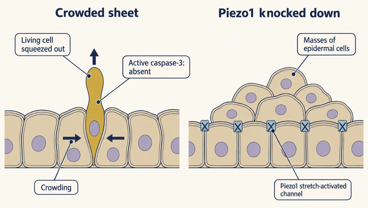
In the first film, the clone’s room came from neighbours that differentiated and left. Space is a second balance alongside m: a basal layer has no spare room, so an extra cell needs a neighbour to leave. Other epithelia show a second exit. Eisenhoffer, Rosenblatt and colleagues counted cells being squeezed out of the sheet (extrusion) in human colon sections, developing zebrafish epidermis and crowded sheets of dog kidney (MDCK) cells. Most lacked active caspase-3, an enzyme switched on in apoptosis, a programmed cell death (see epithelia and cell death). Crowding pushed out living cells, which then died, probably because they lost the survival signals that attachment to the sheet provides. Knocking down Piezo1, a channel opened by membrane stretch, blocked this extrusion in zebrafish and produced masses of epidermal cells.
Predict. In a mouse model of oesophageal carcinogenesis, should more early lesions (small, early tumours) persist, or fewer, if the normal-looking clones around them are made more competitive?
Check your prediction
Fewer. Colom and colleagues found that early lesions were removed more often when the surrounding clones were highly competitive, and less often when competition was blocked with a drug. Competition for space can protect the tissue.
Back to the puzzle
Why can a healthy oesophagus carry so many NOTCH1-mutant cells and not be a tumour? In mouse, losing Notch1 does two things. In normal lining it tilts fate, so clones win space. In a mouse model where oesophageal tumours are induced, deleting Notch1 reduced tumour growth, and a NOTCH1-blocking antibody reduced the size of established lesions. Winning space in normal lining is not the same as growing as a tumour. These are mouse results about mechanism, not human prevention data; which genes do push a clone toward cancer is the subject of cancer genetics and oncogenes.
Winning space changes which cells the lining holds, and that is the idea’s second half: an average over a tissue shifts when its mix of cells shifts. The second film picks up here: what a change in the mix does to a measurement, and how single-cell RNA sequencing sees the mix.
Read the transcript of “The Mix Moves the Average”
Film transcript: The Mix Moves the Average
A bulk RNA reading rises. Did any cell turn the gene up? Chapter one ended on a lining whose mix of cells had changed. Gold clones spread, though on average their cells divided no faster. Now grind that lining up and measure one RNA.
Suppose, with made-up numbers, each gold cell holds 20 copies of one RNA. Each blue cell holds 10. Suppose our bulk assay reports copies per average cell. Early on, gold cells are 2 in 10. Two tenths of 20, plus eight tenths of 10, gives 12 copies per average cell. Later, the clones have spread, and gold cells are 6 in 10. No single cell changes how much RNA it holds. Does the bulk reading go up, go down, or stay the same?
It goes up. Six tenths of 20, plus four tenths of 10, gives 16. The reading rose by a third, yet no cell turned its gene up. Only the mix changed. That is the idea of this lesson. A tissue can change because which cells are there changes, not only because its cells behave differently. On its own, one average cannot tell those apart. To estimate the mix, measure sampled cells one at a time. Single-cell RNA sequencing usually starts by separating tissue into single cells, often with enzymes.
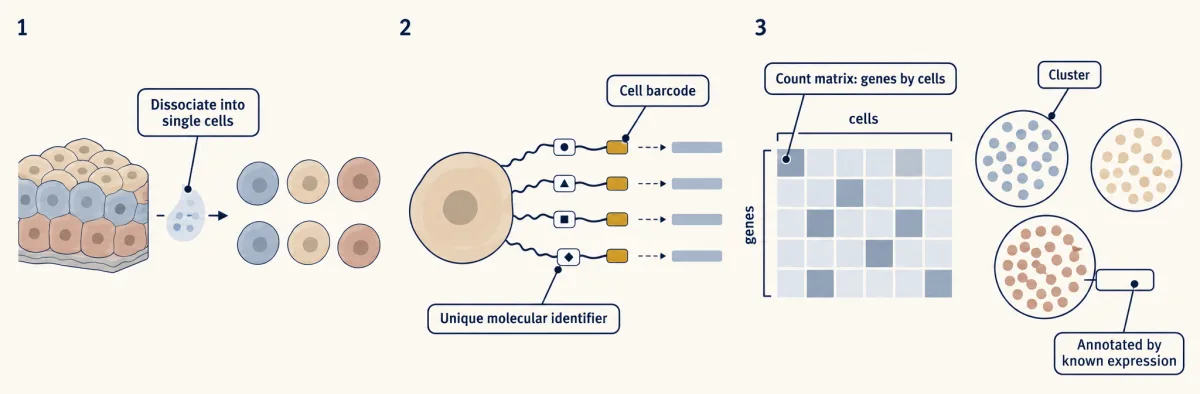
Each captured RNA is copied into DNA carrying a short barcode for its cell. Sequencing produces a count for each gene in each sampled cell. The result is a table, with one row per gene and one column per sampled cell. Software groups cells with similar expression profiles into clusters. Clusters are annotated by comparing their genes with known profiles. Now the shift can be estimated. The gold-profile group contains more sampled cells, while its within-group RNA level stays fixed. But what does a cluster represent? It might mark a cell type, a relatively stable identity such as a keratinocyte or T cell. It might instead mark a state within one type, such as dividing or differentiating. This distinction depends on the question.
Or it might reflect the method. Breaking up tissue can stress cells before capture. Cells from samples processed separately can split by batch. A clustering resolution setting can split or merge groups. A cluster is an observation; what it represents is a hypothesis.
A snapshot cannot reveal ancestry or future fate. Lineage tracing tests those. Perturbation tests cause, and protein can check an annotation. Back in the lining, gold cells became common, so the average moved. No cell made more RNA. Change the mix; the average moves without within-cell change.
From the film
- For amounts expressed per cell, a bulk measurement is a weighted average over the cells in the sample.
- If cell groups differ in per-cell RNA level, changing their proportions shifts that average even when within-group levels stay fixed.
- Single-cell RNA sequencing copies captured RNA into barcoded DNA, produces gene-by-cell counts and clusters similar expression profiles.
- A cluster is an observation that may reflect a cell type, a state or an artifact; what it represents is a hypothesis to test.
Seeing the mixture
In a bulk assay, RNA from all sampled cells is mixed, so an amount expressed per cell is a weighted average over the cell groups. Now try the second film’s arithmetic on a new case.
Predict. Made-up numbers: cell type T expresses gene X at 50 units per cell, other cells at 5. After a treatment, T rises from 20% to 40% of cells, and no cell changes its expression. Does bulk X double?
Check your prediction
No. bulk signal = (fraction T × level in T) + (fraction other × level in other).
- Before: 0.20 × 50 + 0.80 × 5 = 10 + 4 = 14 units per average cell.
- After: 0.40 × 50 + 0.60 × 5 = 20 + 3 = 23 units per average cell.
- Fold change: 23 / 14 = 1.64. A bulk experiment would report gene X up 1.6-fold, although no cell regulated it.
Single-cell data would show the same expression inside each cluster and a changed proportion of clusters.
The rule is exact for amounts per cell; for data normalized per unit of RNA, see Going deeper.
Rule to keep: a bulk change is an average weighted by how many cells of each kind there are, so it can come from a change in composition with no change in regulation in any cell. The numbers are made up, as in the lesson.
Every cell in a tissue carries essentially the same genome, apart from small somatic changes like the mutations above. What makes a keratinocyte differ from a macrophage is which genes it transcribes, a pattern held in place by transcription factors and chromatin (see eukaryotic gene regulation). Single-cell RNA sequencing (scRNA-seq) is one way to read that pattern in sampled cells, as the second film sketched.
The tissue is dissociated into single cells, usually with enzymes. Each captured RNA is copied into DNA tagged with a cell barcode, a short sequence shared by the DNA copies from that cell. The pooled DNA is sequenced (see sequencing and genomes), and reads are sorted by barcode and counted into a count matrix: one row per gene, one column per sampled cell, each entry the number of molecules (with molecular identifiers) or reads counted. Software groups cells with similar expression profiles. Each group is a cluster; comparing its genes with known profiles to propose an identity is annotation.
Single-cell data have their own composition trap: if dissociation loses fragile cells preferentially, cluster proportions are biased before you count, and a shift in cluster sizes between conditions can come from how well each sample survived the enzymes.
Type, state or artifact?
In single-cell data, a change in the sampled mix can appear as a change in cluster sizes, so first ask what a cluster represents. The second film’s line between a cell type (a relatively stable identity) and a cell state (variation within it: cycling, stressed, activated, early or late in differentiation) is a working definition; where the line falls depends on the question and on how finely you look. One cell type can vary a great deal in its global gene expression, and cells of one type in different states can land in separate clusters.
A cluster is an observation to explain, not a type by definition. The second film showed three ways the method can make one; the full list has six, each able to create or erase a cluster, or make one look better supported than it is.
| Artifact | What it does to your clusters | How you would check |
|---|---|---|
| Sampling zeros: only some RNA molecules are captured | A marker looks “missing” from some cells | Do not read one zero as “off” |
| Doublets: one barcode labels two cells | A fake hybrid type with two types’ markers | See the Predict below |
| Batch effects: technical differences between samples processed separately | Cells of one kind split by batch, not biology | Where a population is expected in several samples, check that its cells mix across batches; a real type can be missing from one |
| Dissociation stress: breaking up tissue perturbs state before capture | A stress state made in the dish | Compare with fixed tissue or staining in situ |
| Resolution: a clustering setting for how finely cells are split | Turned up, a type splits into states or noise; turned down, types merge | Check the cluster across resolutions |
| Circular marker testing: clustering on the data, then testing the same data for genes that differ between clusters | Markers look better supported than they are: P values too small, because the clusters were drawn to differ | Confirm with independent evidence, such as protein |
Predict. A small cluster expresses both T-cell genes and epithelial keratin genes. A new hybrid cell type? What would you check first?
Check your prediction
The likeliest reading is a doublet, a T cell and an epithelial cell under one barcode; RNA floating free from broken cells can also contaminate a barcode. Check whether the same barcodes carry both full programmes, whether doublet-detection scores and RNA counts per barcode are high, and whether the cluster’s size fits the rate expected for T-cell–epithelial pairs given how common each type is (not the overall doublet rate). A new type needs independent evidence too.
The 2016 melanoma study of Tirosh and colleagues, 4,645 cells from 19 patients’ tumours, shows the payoff when this is done with care: malignant cells within one tumour differed in programmes associated with the cell cycle, a state rather than a separate cancer type.
From description to cause
The first film followed its clone by a mark every descendant inherited. Single-cell data lack such a mark, so software infers an order: it arranges cells along a path and gives each a pseudotime, its distance along that inferred path from the start. The path is not a movie of one cell maturing. Sequencing destroys each cell, so pseudotime orders different cells caught at different points. Its direction is an assumption, usually set by choosing which end is the start.
Three kinds of evidence test such a picture. Lineage shows ancestry, perturbation tests cause, and protein checks the annotation.
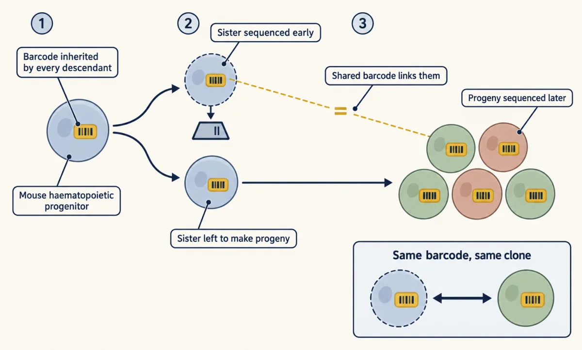
Lineage. Mark a cell and every descendant, as the inducible Cre clones of the mouse experiment did (see stem cells and tissue renewal). Weinreb, Klein, Camargo and colleagues gave mouse blood (haematopoietic) progenitors inherited DNA barcodes that are expressed as RNA, sequenced some cells early and followed their sisters’ progeny. Sister cells shared fate biases that the RNA profiles had not detected.
Perturbation. Remove or block the candidate and see whether the outcome changes, then restore it (see experiments that distinguish mechanisms).
Protein. RNA does not measure protein. CITE-seq, described in 2017, reads DNA-tagged antibodies alongside RNA, so a surface marker can be measured in the same cell rather than inferred.
Going deeper
From counts to clusters
In many methods each molecule also gets a unique molecular identifier, so copies made later can be collapsed back into one original molecule. Analysis then runs through quality control, normalization, choosing informative genes and reducing dimensions. Cells are linked to their most similar neighbours in a graph, and groups of tightly linked cells become clusters. Markers also depend on what else is in the data set. Software such as Monocle builds pseudotime paths.
Weighting by RNA content
If bulk data are normalized per unit of RNA, each type also counts in proportion to its RNA content. Were type T in the worked example to hold twice the total RNA of other cells, the same shift would read about 1.41-fold, not 1.64-fold.
Chance in single clones
In the made-up balanced model, about 15 in 100 labelled clones survive 20 rounds and average about 6.5 progenitors, while the average over all clones stays at 1. Even a tilted clone (m = 1.2) is lost by chance about 43% of the time.
Your notes
Select any text in the lesson to highlight it or add a note to it. Your highlights and notes are saved in this browser and collected in your notebook.
This browser is not letting the site save anything (a private window or strict privacy settings), so highlights and notes will be lost when you leave the page.
How we measure it
Single-cell RNA sequencing
Cells are separated, each cell's RNA is tagged with a cell barcode, and the pooled molecules are sequenced and counted. The result is a matrix of counts, genes by cells, which is clustered and annotated. It measures RNA captured from cells that survived dissociation, not protein and not the cells left behind.
CITE-seq
Antibodies against surface proteins are tagged with DNA oligonucleotides that are read out by sequencing alongside the cell's RNA. One experiment then gives protein and RNA for the same cell, so an annotation does not have to infer surface protein from its RNA.
Inducible Cre lineage tracing
A drug switches on Cre recombinase in a few cells, which both deletes a floxed gene (one flanked by loxP sites) such as Notch1 and turns on a reporter such as YFP. The two sites can recombine independently, so loss of the gene is checked directly, for example by staining for its protein. Every descendant stays labelled, so the size and makeup of each clone can be followed over weeks.
EdU pulse and pulse-chase
EdU, a thymidine analogue, is built into DNA by cells in S phase and detected later by click chemistry. A short pulse gives the fraction of cells in S phase; a pulse followed by a chase shows where the labelled daughters end up, such as still basal or moved upward.
Practice questions on this lesson (3) → MCAT-style, original, each with an explanation
Where this lesson fits
Before thisReview first
- Stem Cells and Tissue RenewalThis course · Lesson 24
You need progenitor and daughter-fate bookkeeping (PP, PD, DD) from there to follow how a clone expands.
- Cyclin-CDK Control of the Cell CycleThis course · Lesson 17
You need to know what division rate means and what drives cycling to separate speed from fate.
- Experiments That Distinguish MechanismsThis course · Lesson 3
This lesson reuses its logic of testing mechanisms by perturbation and ordering of events.
After thisStudy next
- Designing a Cell Biology ExperimentThis course · Lesson 26
You apply the same skill of choosing controls and units to show that one thing caused another.
Elsewhere on the siteFilms, simulations and method films in other courses
- Bomb-pulse carbon-14 dating of cellsMethod film
It dates when human cells were born, a way to measure turnover and renewal in tissue.
- Drift and selection: replicate populationsSimulation · Genetics and Molecular Biology
It shows how random chance in small populations makes some lineages spread and others vanish, like single clones.
Suggested by an AI model from the lessons themselves, then checked. How we use AI
Finish line
Test yourself
8 questions
Practice and MCAT-style, with explained answers.
Next · Lesson 26
Designing a Cell Biology Experiment
Stretched cells glow green. What would it take to show that stretch made them divide?
Continue →