Neuroscience · Unit 6: Cognition and learning
Attention, Executive Control and Decisions
Rewritten on : new text, figures, flashcards and film. Your notes and highlights stay, but the text around them may have moved.
On average, a parietal neuron's firing climbs toward a similar level just before a monkey announces its choice. In one study, silencing that area left the choice no worse. What was the neuron doing?
Pause when the reading reaches a film, and offer to play it. Saved on this device.
Watch the film now, or keep listening
Builds on:Principles of Sensory CodingIntegration, Inhibition and NeuromodulationVisual CortexWhy these?
 ▶ Watch Adding Up Noisy Evidence · 2:17
Read the transcript of “Adding Up Noisy Evidence”
Film transcript: Adding Up Noisy Evidence
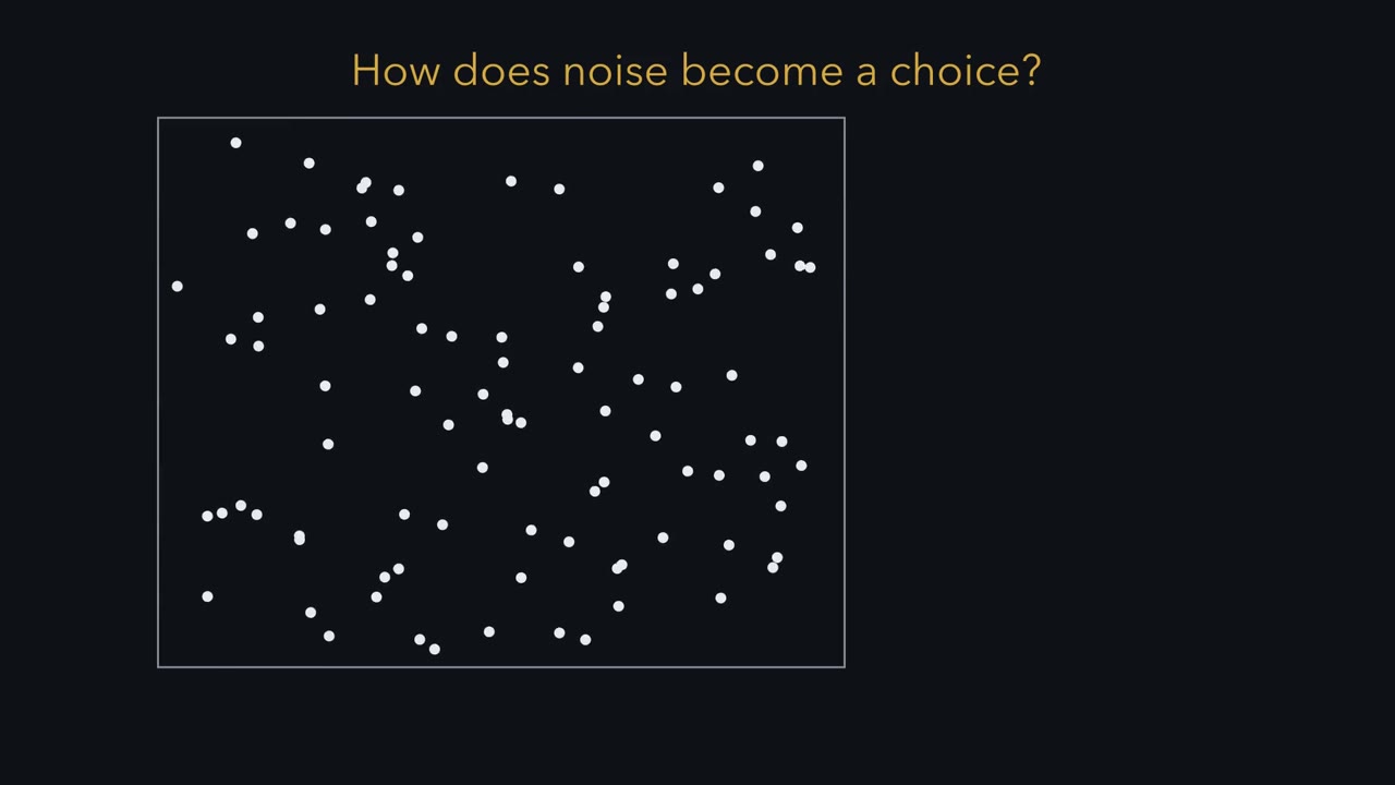
A monkey watches a cloud of moving dots. It must decide which way they are going. How does it turn noise into a choice? Some dots move together, and the rest move at random. The share moving together is called coherence. The monkey answers with a quick eye movement to one of two targets, whenever it is ready. Stronger motion gives faster and more accurate choices. With no net motion at all, the choices fall to chance. Meanwhile, averaged over many trials, a neuron in its parietal cortex fires faster and faster. Is it making the decision? Hold that question. Any single moment of the dots tells you very little. Each glimpse is a weak hint, buried in noise.
So keep a running total. Count each glimpse toward one direction or the other. Hints toward the true direction pile up in step. The random jiggle points every which way, so it partly cancels. Here is a question. You watch four times as long. Is your running total four times as reliable?
No. It is only twice as reliable. The signal grows in step with time. The noise grows too, but only as the square root of time. Assume each glimpse carries the same average signal, with independent noise of the same spread. Reliability here means signal divided by that spread. It grows as the square root of the samples added. That explains the behaviour. Weak motion gives a small push per glimpse, so the total takes longer to become trustworthy. Waiting longer buys accuracy and costs time. So a brain that adds up evidence needs a rule for when to stop. The same arithmetic works across neurons. It helps explain why some effects of attention matter.
The lesson returns to that. Adding up noisy evidence makes it more reliable, because the signal adds in step while the noise partly cancels.
From the film
- Adding up noisy evidence makes it more reliable, because the signal adds in step while independent noise partly cancels.
- Watching four times as long makes the running total only about twice as reliable, because noise grows with the square root of the samples.
- Waiting longer buys accuracy and costs time, so a brain that adds up evidence needs a rule for when to stop.
A monkey watches a cloud of dots, some moving together and the rest at random, and must decide which way the coherent dots are going. As it watches, a neuron in its parietal cortex, toward the top and back of the brain, on average fires faster and faster and reaches a similar level just before the monkey moves its eyes to give its answer.
Is that neuron making the decision? It certainly looks that way. Hold the question; the lesson ends on it. Answering it rests on one piece of arithmetic about deciding under noise. The same arithmetic then helps explain some of what attention does to visual neurons, and the lesson asks where a brain might hold the goal that says what to count.
The task and the puzzle
In the random-dot motion task, a patch of dots appears on a screen. Coherence is the percentage of dots moving together in one direction; the rest move randomly. At 51.2% coherence the motion is easy to see, and at 3.2% it is hard to see. At 0% there is no imposed direction: random fluctuations can favour either side on a given trial, but the expected signal is zero.
Two choice targets sit on either side of the dots. The monkey reports the direction with a saccade (a fast eye movement) to one of them. In the reaction-time version of the task it answers whenever it is ready.
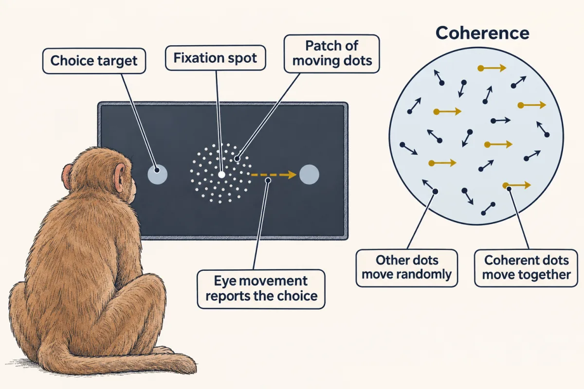
Picture the behaviour as two graphs, each with coherence along the bottom.
- Accuracy (the psychometric curve) rises with coherence. At 0% the choices are at chance.
- Reaction time (the chronometric curve) falls with coherence. Strong motion gives fast answers, and weak motion gives slow ones.
That is the behaviour to explain, and it poses a puzzle. At any one moment the dots give only a weak, noisy hint about the direction. How does a brain turn a stream of unreliable hints into a choice, and why does that take longer when the motion is weak?
The one idea to carry through this lesson. Adding up noisy signals makes them more reliable, because the signal adds in step while independent noise partly cancels.
- Add n samples that each carry the same average push, with independent noise of the same size.
- The signal grows n-fold.
- The noise (its spread) grows only √n-fold, “root n”, the square root of n (see powers).
- So reliability, signal divided by noise, grows as n / √n = √n.
In the drift-to-bound model this lesson uses, a decision is this sum taken over time and stopped at a bound. It is a model of behaviour and of trial-averaged firing; it does not say where in the brain any adding happens, and that gap is the puzzle this lesson ends on.
Why adding up helps
Picture it as a running tally. Each glimpse adds a small push toward the true direction plus a random jiggle. The pushes all point the same way and add in step; the jiggles point every which way and partly cancel.
Predict. You watch four times as long. Is your running total four times as reliable?
Check your prediction
No, twice as reliable. The signal grows fourfold, but the noise grows too, by √4 = 2, so signal divided by noise doubles. In the same way, doubling the viewing time multiplies reliability by √2, about 1.41, not 2.
Two limits keep the rule honest.
- Reliability means signal divided by noise, not percent correct. Percent correct is a bounded, nonlinear function of reliability whose shape depends on the noise and the decision rule, so doubling reliability does not double percent correct. And there must be a signal to add: at 0% coherence waiting cannot help.
- The √n gain needs samples with independent noise. Over neurons, that means only the part of each neuron’s noise that is private to it. Over time, noise that still resembles the last moment’s gives fewer effective independent samples than raw ones, so √t growth is an approximation that holds only under the conditions in Going deeper.
Now the behaviour makes sense. Weak motion gives a small push per glimpse, so the total needs longer to become trustworthy. Waiting longer buys accuracy and costs time. A brain that adds up evidence therefore needs a rule for when to stop.
Adding up evidence: a ramp to a bound
Read the transcript of “A Ramp to a Bound”
Film transcript: A Ramp to a Bound
When should a brain stop collecting evidence and commit to an answer? The evidence comes from MT, the middle temporal area, whose neurons are tuned to direction. What adds it up? The simplest rule is a bound. Keep adding until the running total reaches a set level, then act. Picture a graph, with time along the bottom and the running total up the side. The total drifts upward. Stronger motion means a steeper drift, so the total reaches the bound sooner. Noise adds a wobble. On some trials the total arrives early, and on others late. For a choice between two directions, draw a second bound below the start, for the other answer. On weak-motion trials, the wobble sometimes carries the total to the wrong bound.
That is an error. This is a drift-to-bound model. Suppose some neuron held this running total. What would its firing do just before the eye moves? trials choosing the target this neuron represents, it should climb, more steeply when the motion is strong. And it should reach about the same level just before the eye moves. The other choice has a different endpoint. Now the data. Roitman and Shadlen recorded from the lateral intraparietal area, or LIP, in rhesus monkeys. Its neurons fire before an eye movement to a target in their response field.
Averaged over many trials, the lines lie together for the first 200 milliseconds or so. Then they ramp. The ramp is steeper for stronger motion when the monkey chose the target in the response field. Lined up to the eye movement, the firing reaches about the same rate, whatever the motion strength. The authors read this as an apparent threshold.
These are averages over many trials. Single trials may look different. Noise also changes the timing. At weak motion, the wobble carries many trials to a bound early, sometimes the wrong one. With two bounds, you never wait forever. So mean times are shorter than a noiseless model predicts. Now move both bounds farther from the start. Choices get slower, and more accurate wherever there is net motion.
The slowing is biggest at weak motion, where the wobble, not the drift, sets the time to the bound. A decision can be a running total that stops at a bound. The bound sets the trade between speed and accuracy.
From the film
- In a drift-to-bound model, evidence accumulates until the running total reaches a bound, and stronger motion reaches it sooner.
- In monkey LIP neurons, averaged firing ramps more steeply for stronger motion and reaches about the same rate just before the eye movement.
- Moving the bounds farther away makes choices slower and more accurate, so the bound sets the trade between speed and accuracy.
The evidence comes from MT
The momentary evidence comes from MT, the middle temporal area, a visual area specialized for motion. Its neurons are tuned to direction (see sensory coding). Newsome, Britten and Movshon (1989) found that most of the MT neurons they studied, on a task matched to the neurons’ properties, discriminated motion about as well as, or better than, the monkey. That is a correlation. Salzman, Britten and Newsome (1990) then passed weak electrical current into small clusters of MT neurons with a shared preferred direction (microstimulation) and biased the monkeys’ choices toward that direction. That was a causal test: MT supplies evidence, and in this task its activity can sway the choice. What adds the evidence up?
A rule for when to stop
The simplest rule is a bound: keep adding until the total reaches a set level, then act. Picture it as a line drawn on a graph. Time since the dots appeared runs along the bottom, and the running total runs up the side. The total wobbles but drifts upward, and the model commits to a choice when the total touches the bound. Two features of the picture carry the whole model.
- The drift, the average slope of the total, is set by the strength of the evidence. Stronger motion means a steeper drift, so the total reaches the bound sooner.
- The wobble comes from noise. On some trials it carries the total to the bound early, on others late, so reaction times vary from trial to trial even at one motion strength.
For a choice between two directions, draw a second bound below the starting point for the other answer. The total drifts toward the correct bound, but on weak-motion trials the wobble sometimes carries it to the wrong one. That is an error.
This is a drift-to-bound model (also called bounded accumulation, or drift-diffusion). For the noiseless average, the timing comes out of two lines. The first says how long the climb takes: distance divided by speed.
In words The time to reach the bound equals the distance from the starting level up to the bound, divided by the drift.
- time to bound“time to bound”
- how long the total takes to climb from its start to the bounds
- bound“bound”
- the level of the total at which the model commits to a choiceunits of the total
- starting level“starting level”
- where the total sits when it starts to moveunits of the total
- drift“drift”
- the average slope of the totalunits per second
Sanity check Units: units of the total divided by units per second leaves seconds. Double the drift and the time to bound halves; raise the bound and it lengthens. With zero drift the noiseless total never arrives.
Try one number
Round values to keep the arithmetic easy: a bound 10 units above the start and a drift of 50 units per second. Time to bound = 10 / 50 = 0.2 s.
Double the drift to 100 units per second: 10 / 100 = 0.1 s.
Need a refresher? rates and “per” · units and prefixes
The second line adds the fixed delays on either side of the climb:
reaction time = latency + time to bound + motor delay
The latency is the time before the total starts to move, and the motor delay is the time from reaching the bound to the eye moving. In the model those two are fixed, so only the middle term depends on the drift.
Predict. If some neuron held this running total, what would its firing look like on strong-motion and weak-motion trials? Where would it be just before the eye moved?
Check your prediction
On trials that end at the upper bound, a choice of the target this neuron represents, it should climb, more steeply when the motion is stronger, and reach about the same level just before the saccade whatever the motion strength, because the bound is the same on every trial. Choices of the other target end at the other bound, so they need not reach that level.
The record: LIP
The lateral intraparietal area (LIP) in the parietal lobe holds neurons that fire before an eye movement to a target in their response field. A response field is LIP’s version of a receptive field: the place a target must be for the neuron to fire before a saccade to it. Roitman and Shadlen (2002) placed one of the two choice targets in the recorded neuron’s response field and let rhesus monkeys answer whenever they were ready. Picture their main figure: firing rate against time, one line for each motion strength, averaged over many trials and aligned to the start of motion.
- For the first 200 ms or so the lines lie together: motion strength has not yet shown up in the firing.
- Then they ramp. The ramp is steeper for stronger motion when the monkey chose the target in the response field, and the firing predicts the choice.
- Realigned to the saccade, the lines arrive at about the same rate shortly before the eye moves, whatever the motion strength.
That is what the model predicts for a neuron that holds the total. The authors read the common level as a threshold that appeared to mark the end of the decision. Two cautions. These are averages: whether single trials ramp or step is debated, because a smooth average is compatible with steps of varied timing on single trials, and population recordings are needed to settle it. And LIP firing also mixes in sensory and premotor signals and a rise that grows with elapsed time (an urgency signal), so a common level before the saccade need not mark a pure decision bound.
Worked problem
The numbers are invented for teaching, and one model LIP neuron stands for the accumulator. It fires at 30 spikes/s until 200 ms after motion starts, then climbs. The bound is 70 spikes/s, and the saccade follows 70 ms later. The drift is 400 (spikes/s) per second at 51.2% coherence, 100 at 12.8% and 25 at 3.2%: it scales with coherence.
Step 1, without noise. The distance to the bound is 70 − 30 = 40 spikes/s. The time to bound is 40 / 400 = 0.10 s at 51.2%, 40 / 100 = 0.40 s at 12.8% and 40 / 25 = 1.60 s at 3.2%. Adding the latency and motor delay gives reaction times of 200 + 100 + 70 = 370 ms, 200 + 400 + 70 = 670 ms and 200 + 1,600 + 70 = 1,870 ms. Units: (spikes/s) divided by (spikes/s per s) gives seconds.
Step 2, add the wobble. Real reaction times do not stretch out like that. Add noise and a second bound for the other answer, the same 40 units below the start. A firing rate cannot go below zero, so from here read the total as a relative decision variable, not one neuron’s rate. Choose the noise so that the model is 90% correct at 12.8%: Gaussian, the same size at every coherence (about 60 units per square-root second), with the same 270 ms of latency plus motor delay. The mean reaction times from this model, over both choices, become about 370, 590 and 700 ms. At 0% coherence the mean drift is zero, so only noise reaches a bound: times are long and variable, about 710 ms on average, and the choices fall to chance.
Why does noise make weak-motion answers faster? With two bounds you never wait forever: even with no drift, the wobble carries the total off to one side or the other. At 3.2% the drift alone would take 1.6 s, so the wobble gets most trials to a bound sooner, some of them to the wrong one. Strong motion is unchanged, because the drift does nearly all the work. The small drift is why weak motion gives slow answers; the wobble is why it also gives errors. Turn up the noise in the simulation below to watch this happen (its slider stops at 40, so it shows the effect, not these exact numbers).
Step 3, compare. In one illustrated experiment, Roitman and Shadlen reported a mean of 350 ± 9 ms (SEM) for correct choices at 51.2%. The invented numbers were chosen to land near this, so the match is not a test of the model. The test is the shape: steeper ramps, shorter and less variable reaction times, and higher accuracy as motion strengthens, all from one rule.
The speed–accuracy trade
Raise the bound and every trial must gather more evidence. Choices get slower and more accurate wherever there is net motion; at 0% they stay at chance. In the noisy model the slowing is largest at weak motion, because there the wobble, not the drift, sets how long the total takes to reach a bound. In the worked problem’s model, moving both bounds 10 units farther from the start (the upper one from 70 to 80) adds about 25 ms at 51.2% coherence, 120 ms at 12.8% and 230 ms at 3.2%.
- The lesson’s arithmetic
- —
- Noiseless reaction time (expected)
- —
- Observed mean, noisy trials
- —
- Expected mean for this noisy sketch
- —
- Choices toward the preferred target
- —
—
In this sketch: invented numbers (30 spikes/s baseline, 70 spikes/s bound, 200 ms latency, 70 ms motor delay), one neuron standing for the accumulator, no noise unless you set it. With noise, the accumulator takes random steps in relative units and a second bound for the other choice sits 40 relative units below the baseline, symmetric with the upper bound, which is why it can fall below 0 on this relative scale. Time is cut off at 3 s on the plot; noisy trials are run to 6 s. Expected means and choice percentages are the standard first-passage results for this random walk between two bounds, not figures from the lesson.
rise time = (bound − baseline) / slope, and reaction time = latency + rise time + motor delay. The ramps in the lesson are trial averages, and whether single trials ramp or step is debated; this sketch draws a noisy accumulator and does not settle that.
How long to keep sampling also depends on what a choice is worth, which links to motivation and reward, and selecting one action among many draws on the basal ganglia.
Attention: a stronger signal, less shared noise
Return to the rule, now across neurons instead of across time. Each neuron is like one glimpse, so a downstream cell that adds up many neurons gains in the same way: their private noise partly cancels, their shared noise does not, and a stronger signal helps either way. Attention acts on both.
Attention is selecting part of what is available for further processing. Keep it apart from arousal, the overall level of alertness, which shifts with sleep and rhythms. A receptive field is the region of space in which a stimulus changes a neuron’s firing, as in visual cortex. V4 is a mid-level visual area in the macaque.
Attention biases a competition
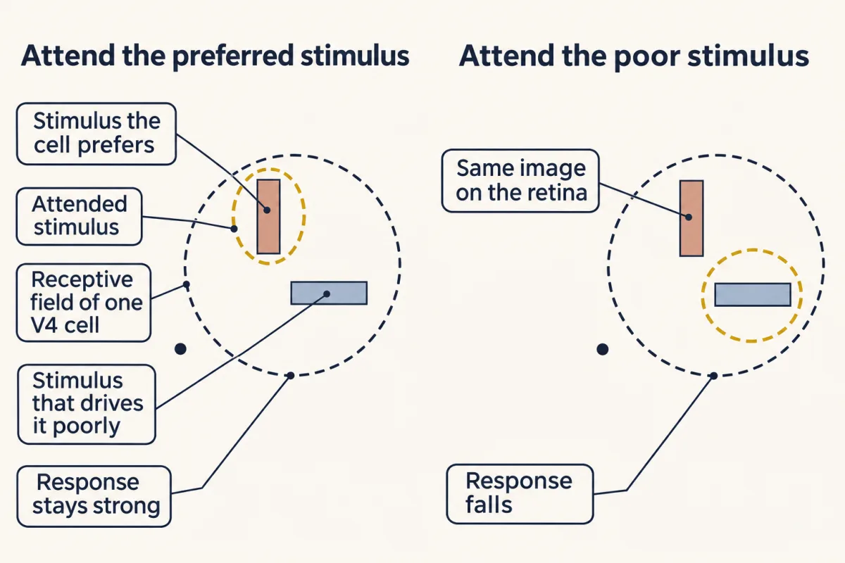
Moran and Desimone (1985) recorded from neurons in macaque V4 and placed two stimuli inside one receptive field: one that drove the cell well and one that drove it poorly. Then they changed only where the monkey attended.
Predict. The monkey attends to the stimulus the cell responds to poorly. Does the response go up, go down, or stay the same?
Check your prediction
It goes down. When the monkey attended to the poor stimulus, the response fell toward what that stimulus gave alone, although the retinal image was unchanged.
Stimuli seem to compete for a neuron, and attention biases the competition toward the attended one. In that study, primary visual cortex (V1) cells showed no such effect; later work found smaller attention effects there.
Attention acts like more contrast
Picture a contrast-response curve: a neuron’s response on the vertical axis against stimulus contrast on the horizontal. It rises steeply at low and middle contrasts, then flattens near the top, where responses saturate.
Reynolds, Pasternak and Desimone (2000) varied contrast and found that attention raised V4 responses more at low contrast than at high. On average, attention acted as if it multiplied the stimulus contrast by 1.51. An attended 10% contrast grating drove cells about as well as an unattended grating of 10 × 1.51 ≈ 15%. Draw the attended curve on a contrast axis with a log scale and it is the same curve slid to the left. So the same multiplication raises the response most where the curve rises steeply and hardly at all near saturation. This pattern is called contrast gain. Response gain, a separate pattern other studies have reported, scales the whole curve up instead; the turning-up-the-volume picture in the Like-I’m-five summary is closer to it. In terms of the rule, contrast gain is a stronger signal for the attended stimulus.
Attention lowers shared noise
Attention also changes how neurons vary together. Show the same stimulus many times and count two neurons’ spikes on each repeat. Plot one count against the other, one dot per repeat. If the two tend to fire more on the same repeats, the cloud of dots tilts; if not, it has no tilt. Noise correlation is the correlation of two neurons’ spike counts across repeats of the same stimulus:
ρ = Cov(n1, n2) / √(Var(n1) × Var(n2))
Read it as: ρ (“rho”) is how much the two counts move together (their covariance, Cov), scaled by the two counts’ own variability (the square root of the product of their variances, Var), so that it runs from −1 to +1. Here n1 and n2 are the two neurons’ spike counts; this n is a count, not the number of samples from the one idea above.
How much does that shared noise matter when a downstream cell averages many neurons? The guiding rule gives the answer:
In words The variance of the average equals sigma squared, times one plus N minus one times rho, all divided by N.
- variance of the average“variance of the average”
- the spread of the pooled signal across repeats; its square root is the pooled noisespikes²
- σ²“sigma squared”
- one neuron's noise variance. σ (sigma) is the noise size, its square root.spikes²
- N“N”
- the number of similarly tuned neurons averagedno unit
- ρ“rho”
- the pairwise noise correlation between neuronsno unit
Sanity check With ρ = 0 the bracket is 1, the variance is σ²/N, and the noise of the average shrinks as 1/√N. With ρ above zero, the private part still shrinks, but the shared part stays. As N grows, the bracket over N approaches ρ, so the noise falls toward a floor of σ√ρ, and pooling can improve on one neuron at most 1/√ρ-fold.
Try one number
Round values, chosen only to keep the arithmetic easy: N = 4 neurons with ρ = 0.5.
Bracket: 1 + (4 − 1) × 0.5 = 2.5. Variance: σ² × 2.5 / 4 = 0.625σ². Noise (the square root): √0.625 ≈ 0.79σ.
With ρ = 0 the variance would be σ²/4 and the noise σ/2. With ρ = 0.5 the pooled noise is 0.79σ, not 0.5σ: shared noise cannot be averaged away.
Where it comes from optional
Optional: where it comes from. The variance of a sum of N counts is the sum of their N variances, σ² each, plus all N × (N − 1) covariances (one for each ordered pair of different neurons), ρσ² each. That gives σ² × [N + N(N − 1)ρ].
An average is the sum divided by N, which divides the variance by N². So the variance of the average is σ² × [N + N(N − 1)ρ] / N² = σ² × [1 + (N − 1)ρ] / N.
Need a refresher? powers and roots · rates and “per”
Predict. Average 100 neurons whose noise correlation is 0.065. How much less noisy is the average than one neuron? What if the correlation were zero?
Check your prediction
With ρ = 0.065, the variance of the average is σ² × (1 + 99 × 0.065) / 100 ≈ 0.074σ², so the noise is about 0.27σ: about 3.7 times smaller than one neuron’s. With ρ = 0 it would be σ/10, ten times smaller. Even an endless pool could do no better than 1/√0.065, about 3.9-fold. A small shared correlation wipes out most of the benefit of a large pool.
Kanashiro and colleagues (2017) reanalyzed V4 recordings from two monkeys detecting orientation changes. Mean noise correlation was 0.065 unattended and 0.045 attended. As an illustration, in an idealized pool of 100 identical, similarly tuned neurons, that drop would cut the pooled noise by about 14%, even though each neuron’s own variability rose slightly. That is a calculation from the averages, not a measured pool. So for a readout that adds up similarly tuned neurons, less shared noise makes the pool more reliable. For other readouts, whether a correlation hurts depends on how it lines up with the neurons’ tuning; some correlations are harmless, or even helpful, for an optimal decoder.
Where does the bias come from? Attention also depends on parietal and frontal cortex, as damage in humans shows. After damage there, a patient may fail to notice or respond to things on the side of space opposite the lesion (contralesional hemispatial neglect). Neglect is commoner and more severe after right-hemisphere damage.
Holding the goal: prefrontal cortex
Attention needs a target, and a decision needs to know which evidence counts. One answer to what sets them points to the front of the brain.
Executive control is the ability to organize thought and action according to internal goals rather than whatever the senses offer next. Working memory, holding information that is no longer in front of you so that you can use it, is one of its tools. Both are tied to the prefrontal cortex, the front part of the frontal lobe, which never works alone. Working memory is different from the long-term stores in memory systems.
Holding a place in mind
The classic recording came from monkeys. Funahashi, Bruce and Goldman-Rakic (1989) trained them in an oculomotor delayed-response task. The monkey fixated a central spot, a cue flashed for 0.5 s at one of several peripheral places, and the monkey kept fixating through a delay of 1 to 6 s before making a saccade to where the cue had been.
Fixation is the key control. With the eyes still and the screen blank, firing that depends on the cue’s location cannot be a response to a visible cue or to an eye movement under way. Fixation does not rule out a movement being planned, though. Whether delay activity is a memory of the place or a plan to look there is a question this task alone cannot settle.
The recordings came from around the principal sulcus, a groove in the lateral prefrontal cortex. Of 288 neurons, 87 changed their firing in the delay and 79% of those were directionally selective: 0.79 × 87 ≈ 69 cells, about 24% of the sample, carried the remembered direction through the delay. A subset of principal-sulcus neurons did this, in this task, in monkeys.
Holding a rule
Prefrontal neurons also code what to do. Wallis, Anderson and Miller (2001) trained monkeys to judge two pictures under one of two rules, respond if they match or respond if they differ. The most common activity in their prefrontal sample reflected the rule in force, and the monkeys applied the rules to pictures they had never seen. The new pictures matter: a cell that signals the rule for a novel picture cannot be signalling a memorized picture-response pairing.
A theory that ties these together
Miller and Cohen (2001) proposed that prefrontal cortex maintains representations of goals, and these bias processing in other structures toward what the goal needs. Think of a coach on the sideline who holds the plan. The players do the running, but the coach’s call tips which play the team runs. In this lesson’s terms, the goal says which signal to count. That is not a claim that prefrontal cortex does the adding. It is a proposal, and the prefrontal cortex is one partner among several.
When the best correlate is not necessary
Read the transcript of “Visible Is Not the Same as Needed”
Film transcript: Visible Is Not the Same as Needed
LIP firing looks like the running total. But does the decision actually need LIP? A recording shows what activity goes with a choice. Only changing the activity can test whether the choice depends on it. MT passed a first test. Researchers passed weak current into small clusters of MT neurons that shared a preferred direction. The monkeys chose that direction more often, as if that motion had been added to the dots. Katz, Yates, Pillow and Huk then silenced each area in turn, in rhesus monkeys. They used muscimol, a drug that activates GABA-A receptors and quiets nearby neurons. Predict each outcome. If LIP is the accumulator, what happens when you silence MT?
And when you silence LIP? Silencing MT impaired motion discrimination. Silencing LIP produced no measurable impairment of the motion decisions, in the tasks tested. Did the injection simply miss? The same monkeys did a free-choice task, with no right answer. After LIP inactivation, they chose targets in the affected part of space less often. And their eye movements to that side landed less accurately. So the drug had acted on LIP. That control is what makes the null result readable. Still, a null result cannot rule out other areas compensating. Other studies did find deficits after parietal inactivation. So the result is debated. In one study, the biases faded while the area was still silenced.
That suggests other areas compensated. Which areas a decision needs remains an open question. If a decision adds up evidence, the adding happens somewhere, perhaps in several places. But a neuron that shows the running total is not always the place it is needed.
From the film
- A recording shows what activity goes with a choice, and only changing the activity can test whether the choice depends on it.
- In monkeys, silencing MT impaired motion discrimination, but silencing LIP produced no measurable impairment in the tasks tested.
- A null result cannot rule out compensation by other areas, and other studies found deficits, so which areas a decision needs remains open.
Go back to the neuron in the opening. LIP firing looks like the running total. But correlation shows only what activity goes with a choice. A manipulation asks two further questions: does changing the activity change the choice, and does the choice need it? MT passed the first test when stimulation swayed the choice in this task. Does the choice need MT, or LIP?
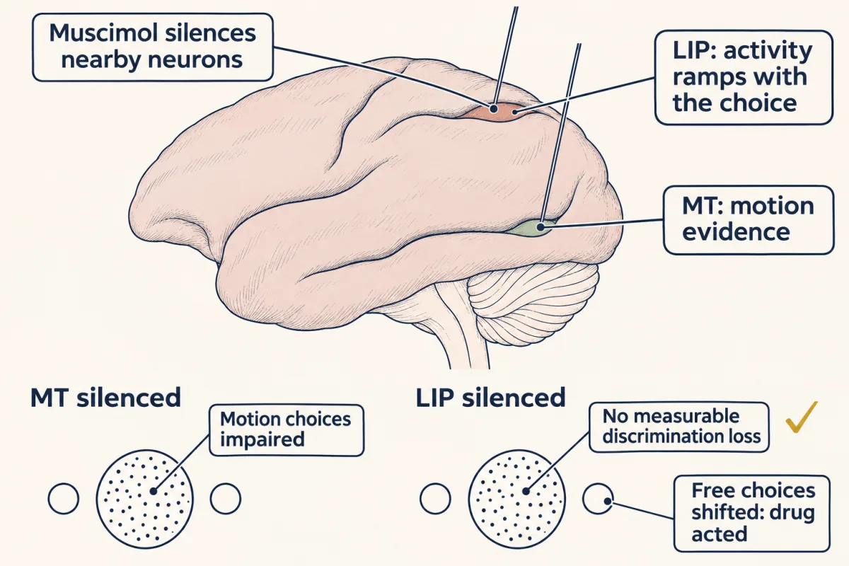
Katz, Yates, Pillow and Huk (2016) recorded MT and LIP in rhesus monkeys and then reversibly silenced each with muscimol, a drug that activates the inhibitory GABA-A receptors (see synaptic transmission) and quiets nearby neurons.
Predict. If LIP is the accumulator, what should happen to motion discrimination when MT is silenced? When LIP is silenced?
Check your prediction
If LIP were the one place the evidence is added up, and nothing else could cover for it, silencing either area should impair discrimination. In fact MT inactivation impaired motion discrimination, but LIP inactivation produced no measurable impairment of motion decisions in the tasks tested.
A null result is easy to dismiss: perhaps the injection missed, or was too small. So the same monkeys did a free-choice task with no right answer. After LIP inactivation they chose targets in the affected part of space less often, and their saccades to that side landed less accurately, so the drug had acted. The control is what makes the null result readable. Even so, a null result cannot exclude compensation by other areas.
What other studies found. The result is debated.
- Microstimulation of LIP has biased choices (Hanks, Ditterich and Shadlen, 2006).
- Zhou and Freedman (2019) found that parietal inactivation impaired motion and category decisions, most when the visual stimuli, rather than the response targets, sat in the inactivated field.
- Jeurissen and colleagues (2022) found that LIP inactivation biased decisions, but the biases faded while the area was still silenced, which suggests that other areas compensated.
The model survives: if a decision is built by adding up evidence, the adding is done somewhere, perhaps in several places at once. What the experiments show is that a neuron displaying the running total is not thereby the place the total is needed. Which areas a decision needs, and whether that changes with training and task, is an open question.
Design problem
Muscimol in MT raises the motion-discrimination threshold; in LIP it leaves the threshold unchanged, though monkeys choose targets in the inactivated field less often in a free-choice task. What does this say about LIP as “the accumulator”, and what would you do next?
Saved in this browser only.
One way to do it
LIP activity correlates with the decision, but silencing the targeted LIP sites caused no measurable discrimination deficit under these conditions. The free-choice effect shows the inactivation worked, so the null result is not a missed injection. It does not rule out a contribution that spared tissue or other areas could cover. MT was needed for this discrimination, as expected of a stage that carries direction evidence, though direction-selective signals already reach MT from V1.
Several readings remain. Other areas that carry choice signals, such as the frontal eye field or the superior colliculus, may hold the signal redundantly or compensate when LIP is silenced. Or LIP may reflect a decision computed elsewhere. Next, inactivate several areas together, and record many neurons at once to see single-trial dynamics. Scope every conclusion to this task, this training and this species. The circuit experiment design and large-scale neuroscience lessons build those tools.
Going deeper
The numbers behind the worked problem
The drifts in the worked problem come from one constant: 7.8125 (spikes/s) per second for each percent coherence, which makes 51.2% come out at exactly 400. The simulation uses the same constant.
When adding up stops helping
The exact √n rule applies to independent samples with the same expected signal and finite noise variance. If the noise drifts slowly, so that one moment’s noise resembles the last, adding the two cancels little. The span over which it still resembles the last is the noise’s correlation time, and over windows shorter than that, waiting barely helps. For steady (stationary) noise with a stable mean signal whose correlations die away fast enough to have a finite integrated autocovariance, adding over windows much longer than the correlation time gives approximately √t growth in reliability, with fewer effective independent samples than raw ones. A long window is an approximation, not a guarantee of independence: slowly decaying correlations, or noise shared across a whole trial, prevent the gain.
The Kanashiro figures
In Kanashiro and colleagues’ reanalysis, mean covariance fell 34.0% while mean single-neuron variance rose 1.61%. Dividing one by the other does not reproduce the mean correlations (0.065 × 0.66 / 1.016 ≈ 0.042, not 0.045), presumably because the paper averaged pair by pair, so do not try to recompute one from the other. The 14% illustration in the main text comes out the same to the nearest percent with or without the small rise in variance (13.7% with it, 14.3% without). Their circuit model predicts that attention acts mainly on inhibitory neurons, a prediction still to be tested.
Holding a goal: thalamus and prefrontal cortex in mice
In mice running a delayed non-match-to-sample task in a T-maze, Bolkan and colleagues (2017) inhibited pathways selectively. Input from the mediodorsal thalamus (a thalamic nucleus, or cluster of neurons, connected with prefrontal cortex) to medial prefrontal cortex supported maintenance during the delay, and the reverse projection supported the later choice. Delay firing in medial prefrontal cortex needed the thalamic input, yet those delay-tuned neurons overlapped minimally with neurons tuned to position in the maze.
Memories that go quiet
In humans, Rose and colleagues (2016) cued people to set one remembered item aside. That item’s category could no longer be decoded from the electroencephalogram (EEG), but a single TMS pulse briefly made it decodable again, and only while it might still be needed. The authors suggest that short-term synaptic changes could hold such latent items. The synapses were not measured, and because decoding was at the category level, reinstated category context is an alternative to reactivation of the item itself.
Your notes
Select any text in the lesson to highlight it or add a note to it. Your highlights and notes are saved in this browser and collected in your notebook.
This browser is not letting the site save anything (a private window or strict privacy settings), so highlights and notes will be lost when you leave the page.
How we measure it
Single-neuron recording in behaving monkeys
A microelectrode records the spikes of one neuron while a trained monkey performs a task with controlled stimuli, delays and responses. Aligning spikes to events (cue, motion onset, saccade) shows what the neuron's firing goes with, which is a correlate, not a cause.
Electrical microstimulation
Weak current pulses through an electrode activate neurons and axons near the tip. In MT, nearby neurons share a preferred direction, so a site can be chosen for its tuning. If behaviour shifts in the direction those neurons prefer, as in MT during motion judgments, their activity can influence the choice in that task.
Reversible pharmacological inactivation
A small injection of muscimol, a GABA-A receptor agonist, silences neurons near the tip for a limited time. A deficit shows the area contributes to that task. No deficit means no effect was detected under those conditions, which is informative only if a control shows the drug worked; other areas may still compensate.
TMS with EEG decoding
A classifier trained on EEG patterns reads out which category of item (not the individual item) a person is holding in memory; a transcranial magnetic stimulation pulse perturbs cortex noninvasively. Together they can probe whether an item that cannot be decoded is still stored in a latent form.
Practice questions on this lesson (3) → MCAT-style, original, each with an explanation
Where this lesson fits
Before thisReview first
- Principles of Sensory CodingThis course · Lesson 9
You need how neurons' firing rates encode stimulus features, such as MT direction tuning, to follow the evidence that gets added up.
- Integration, Inhibition and NeuromodulationThis course · Lesson 7
Summing many inputs, including inhibition, is the neural version of the adding-up rule used here.
- Visual CortexThis course · Lesson 11
V4, receptive fields and MT motion areas build on how visual cortex is organized and tuned.
After thisStudy next
- When Mature Neurons Fail: NeurodegenerationThis course · Lesson 26
It repeats the question of reading absolute against relative effects in noisy outcome data, taking this lesson's evidence logic further.
- Designing a Causal Circuit ExperimentThis course · Lesson 28
It takes the correlate-versus-necessary question further, using causal tests such as silencing and light in circuits.
Elsewhere on the siteFilms, simulations and method films in other courses
- Weighting two senses by reliabilitySimulation · Sensory Systems
It uses the same reliability-weighted adding of noisy evidence, with each sense weighted by its variance.
- Which Sense Do You Believe?Film · Sensory Systems
It shows how noisy signals are combined by their reliability, the same arithmetic as adding up evidence.
Suggested by an AI model from the lessons themselves, then checked. How we use AI
Finish line
Test yourself
8 questions
Practice and MCAT-style, with explained answers.
Next · Lesson 26
When Mature Neurons Fail: Neurodegeneration
Lecanemab slowed worsening in early Alzheimer disease by about 27%. The treated group still got worse.
Continue →