Neuroscience · Unit 2: Synapses and plasticity
Synaptic Transmission and Quantal Release
Rewritten on : new text, figures, flashcards and film. Your notes and highlights stay, but the text around them may have moved.
A resting frog muscle fibre shows small voltage blips at its endplate with no nerve impulse at all. Those blips are the units of the evoked response at this junction.
Pause when the reading reaches a film, and offer to play it. Saved on this device.
Watch the film now, or keep listening
Builds on:The Resting Membrane and Passive SignalsThe Action Potential and ConductionWhy these?
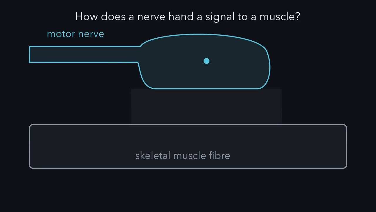 ▶ Watch Blips from a Silent Nerve · 2:38
Read the transcript of “Blips from a Silent Nerve”
Film transcript: Blips from a Silent Nerve
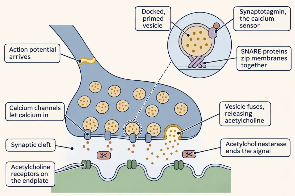
How does a nerve hand a signal to a muscle? And what is that signal made of? A synapse is a site where one neuron passes a signal to another cell. At a chemical synapse, the terminal releases a transmitter. It crosses a gap and acts on receptors. The best-studied example is the junction between a motor nerve and a skeletal muscle fibre. The signal crosses in a relay of five steps. For now, the names are enough. First, an action potential arrives at the nerve terminal. Second, calcium flows into the terminal. Third, vesicles fuse with the membrane and release their transmitter, acetylcholine. Fourth, acetylcholine crosses the gap. Fifth, it opens receptor channels on the muscle fibre, and the fibre depolarizes.
That depolarization is the endplate potential. The endplate is the patch of fibre under the terminal. Now the record that started the story. Paul Fatt and Bernard Katz put a fine glass electrode inside a frog muscle fibre. Voltage runs up the side. Time runs along the bottom. They did not stimulate the nerve at all. So the trace should be flat. Mostly it is. But small blips rise from it at irregular moments. Each blip is about the same size. Each is far too small to fire the fibre. Move the electrode away from the endplate, and the blips shrink and fade. So Fatt and Katz attributed them to acetylcholine released spontaneously by the terminal.
They called them miniature endplate potentials, and reported them in 1952. Each miniature looked like a scaled-down copy of the response the nerve evokes. Here is the puzzle. Is the nerve's real response built from blips like these?
It is. The evidence comes in the next chapter. That answer raises more questions. How do you count units that merge together? Why does calcium matter so much? What sets the size of one unit? And how can a recording tell which side of a synapse is at fault? The miniature is the unit. Every evoked response at this junction is built from it.
From the film
- A nerve passes a signal to a muscle fibre in a relay: terminal impulse, calcium entry, vesicle release of acetylcholine, then receptor channels opening.
- A resting frog muscle fibre shows small blips with no nerve impulse, which Fatt and Katz attributed to acetylcholine released spontaneously.
- The miniature is the unit from which the evoked response at this junction is built.
Put an electrode inside a resting frog muscle fibre at the point where the nerve ends, stimulate nothing, and you still see small depolarizations arriving at random, each about the same size and each far too small to fire the fibre.
Paul Fatt and Bernard Katz reported these miniature endplate potentials in 1952. They turned out to be the bricks from which every nerve-evoked response at that junction is built.
The relay and the blips
A synapse is a site where one neuron passes a signal to another cell. At a chemical synapse the presynaptic terminal releases a transmitter that crosses a gap, the synaptic cleft, and acts on receptors of the postsynaptic cell. The vertebrate neuromuscular junction, where a motor axon meets a skeletal muscle fibre, is the best-studied example. How it is built during development belongs to the neuromuscular junction in Developmental Neuroscience, along with central synapses and synapse elimination.
The sequence runs like a relay with five steps:
- An action potential arrives at the nerve terminal.
- Calcium flows into the terminal.
- Synaptic vesicles fuse with the terminal’s membrane and release their transmitter, acetylcholine.
- Acetylcholine crosses the cleft.
- Acetylcholine opens receptor channels on the muscle fibre, and the fibre depolarizes.
That depolarization is the endplate potential (EPP), the muscle’s version of an excitatory postsynaptic potential (EPSP), a depolarization caused by transmitter. The endplate is the region of the muscle fibre that lies under the nerve terminal.
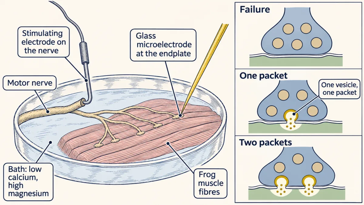
Now picture the record that started the story. Fatt and Katz put a fine glass electrode inside a frog muscle fibre at the endplate. Voltage runs up the side and time along the bottom. With no stimulus to the nerve, the trace should be flat. It is flat most of the time, but blips rise from it at irregular moments. Move the electrode away from the endplate and the blips shrink and fade.
Fatt and Katz called these miniature endplate potentials, or miniatures. They looked like scaled-down copies of the evoked endplate potential, so Fatt and Katz attributed them to spontaneous release of acetylcholine from the terminal.
The record raises five puzzles, and this lesson answers them in order.
- Units. Is the nerve’s evoked response built from blips like these?
- Counting. If it is, how can you count units that merge into one smooth response?
- Calcium. Why does release depend so steeply on calcium?
- Size and safety. What sets the size of one unit, and how far above threshold does a normal response sit?
- Disease. Two diseases both weaken muscle. How do you tell from a recording which side of the synapse is at fault?
Packets: turning release down
Read the transcript of “Turn Release Down to See the Packets”
Film transcript: Turn Release Down to See the Packets
If the nerve's response is built from miniatures, why can't you just see them? In normal calcium, one impulse releases dozens of units or more at once. They merge into one smooth response. It is like a downpour, where you cannot count the drops. To count drops, you need a drizzle. So del Castillo and Katz lowered calcium and raised magnesium in the bath around a frog junction. That cut release to a trickle. Now an impulse often produced nothing at all. That is called a failure. When a response did come, it was small. So they stimulated many times and sorted the sizes. Picture a histogram. Response size runs along the bottom. The number of trials runs up the side.
If release were a smooth flow, just turned down, what shape would this histogram have? One simple smooth-flow model would give one smooth spread of sizes, with no regularly spaced peaks. The telling sign of packets would be peaks spaced at one miniature. That is not what they found. Watch the trials drop in. A tall bar builds at zero. These are the failures. A bump grows near the size of one miniature. The miniature histogram lines up over it. A smaller bump grows near twice that size. A smaller one again near three times. The bumps are broad, because one unit is not exactly the same size every time, and the recording has noise. But the sizes cluster near whole-number multiples of the miniature.
The response comes in packets. Each packet is called a quantum. Its effect on the muscle, the miniature, is the quantal size, A quantum holds thousands of acetylcholine molecules. It was later tied to the contents of one vesicle. It is not one molecule. Think of coins dropped into a jar on a scale. You cannot see the coins. But if every reading is a multiple of one coin's weight, you can count them.
That gives the one idea of this lesson: each response ≈ count × size. The nerve terminal sets the count, Calcium sets it steeply. One vesicle's transmitter, acting on the receptors, sets the size, Big responses fall short of this rule. A later chapter shows why. The count is random from impulse to impulse. What we track is its average, So when transmission changes, ask first. Did the count change, the size, or both?
From the film
- In normal calcium the units merge into one smooth response, so release has to be turned down to see them.
- In low calcium and high magnesium, responses cluster near whole-number multiples of the miniature, with failures at zero.
- Each response is roughly count times size, so when transmission changes, ask whether the count, the size or both changed.
Del Castillo and Katz asked whether the evoked response was made of the same units as the miniatures. In normal calcium that is hard to see. One impulse releases dozens of units or more at once, and they merge into one smooth response, like a downpour where you cannot count the drops. To count drops you need a drizzle.
So they bathed the frog junction in a solution with less calcium and more magnesium, which cut release to a trickle. Now a nerve impulse often produced nothing at all, a failure. When it did produce a response, the response was small. Stimulate many times, and sort the response amplitudes into a histogram.
Predict. Suppose release were a smooth flow that the low calcium simply turned down. What shape would the histogram of response amplitudes have?
Check your prediction
In one simple smooth-flow model, with sizes spreading around a small average and no all-or-none step, you would expect one smooth spread with no peaks at regular spacing. That is only one alternative: continuous release alone neither fixes the shape nor rules out failures. The telling evidence would be peaks spaced at multiples of one miniature.
That is what they found. Picture the histogram. Response amplitude runs along the bottom, and the number of trials with that amplitude runs up the side.
- A tall bar at zero. These are the failures.
- A bump near the size of one miniature. Lay the histogram of spontaneous miniatures over it, and the two line up.
- A smaller bump near twice that size, and a smaller one again near three times.
The bumps are broad, not sharp spikes, because one unit is not exactly the same size every time and the recording has noise. But the amplitudes cluster near whole-number multiples of the miniature. The evoked response came in packets.
Each packet is a quantum, and its postsynaptic effect, the miniature amplitude, is the quantal size, q. A quantum is a multimolecular packet, thousands of acetylcholine molecules, later identified with the contents of one vesicle. It is not one molecule of acetylcholine.
Think of coins dropped into a jar on a scale. You cannot see the coins, but if every reading is a multiple of one coin’s weight, you can count them.
The one idea to carry through this lesson. Every evoked response is a whole number of near-identical packets, so each response ≈ count × size, and on average EPP ≈ m × q, where m is the average count. The nerve terminal sets the count, and calcium sets it steeply. One vesicle’s transmitter acting on the receptors sets the size, q. So a change in transmission at this junction can be asked one question first: did the count change, the size, or both?
Three limits come with it. Big responses fall short of count × size (the section on packet size shows why). The count is random from impulse to impulse, so single responses scatter around the average. And with the muscle membrane and the recording held steady, the size depends on two things, how full the vesicle is and how many receptors face it, so a change in q alone does not say which side of the synapse moved.
Counting quanta you cannot see
Read the transcript of “Counting with Zeros”
Film transcript: Counting with Zeros
How do you count packets when the bumps blur together? You want one number: the mean quantal content, It is the average number of packets one impulse releases. There are two ways to get it. They rest on different assumptions, and that is the point. The first is direct. Every response is a whole number of packets. So the average response, divided by the size of one packet, gives the average count. Count each failure as a response of zero. This needs evoked packets the same size as miniatures, and packets that add linearly. The second way sounds like a trick. It counts only the failures. Picture the terminal as a row of release sites, like tiny lamps.
On each impulse, every site has a small chance to flash, independently of the others. A flash is one packet released. A failure means every single site stayed dark. The more packets released on average, the rarer an all-dark trial becomes.
Each site stays dark with chance one minus p. The sites are independent, so multiply those chances together. When p is small, that product comes very close to e^(−m). So the fraction of failures fixes the average count. The formula is on screen. Suppose an impulse releases one packet on average. How often does it release nothing at all?
More than a third of the time. The number is on screen. The average is pulled up by trials that release two or three. Why bother with two methods? Because the failure method never uses the size of a packet. If evoked packets differed in size from miniatures, the direct method would go wrong. The failure method would not, as long as failures can still be told apart from noise. So when the two estimates agree, that agreement supports two things. That evoked and spontaneous packets are the same units, and that release behaves like many small, independent chances. In a made-up recording of two hundred stimuli, the two estimates both come out near one packet.
The same reasoning predicts how many trials release each number of packets. That is the Poisson distribution. Each site's chance must be small. Small, not equal. Now restore normal calcium. The total release becomes large, tens of packets on every impulse. Failures vanish, so there is nothing left to count. Low calcium is what makes failures common enough to measure. Low calcium is not just convenient. It makes the chances small and failures common, as the mathematics needs.
From the film
- The mean quantal content can be found two ways: average response divided by packet size, or from the fraction of failures.
- The failure method never uses packet size, so agreement between the two supports evoked and spontaneous packets being the same units.
- Low calcium makes failures common enough to count, which the mathematics needs.
The histogram shows packets, but in most recordings the bumps blur together. What you want is one number, m, the mean quantal content. (This is not the m of Hodgkin and Huxley’s gates in the action potential lesson; the two fields happen to use the same letter.) There are two ways to get it. They rest on different assumptions, so if the model is right, the two estimates should agree within sampling error.
The direct way: divide the average response by one packet
If every response is count × size, then dividing the average response by the size of one packet gives the average count. Rearrange the rule EPP ≈ m × q (divide both sides by q), counting each failure as a response of zero when you take the average:
In words The mean quantal content is the average evoked response, failures counted as zero, divided by the average size of one spontaneous packet.
- m“m”
- the mean quantal content: the average number of packets released per impulsepackets
- mean EPP“mean E P P”
- the average endplate potential over all stimuli, with each failure counted as 0mV
- mean miniature“mean miniature”
- the average size of one spontaneous miniature, the quantal size qmV
Sanity check The millivolts cancel, so m is a pure count. If the average response equals one miniature, m = 1. If evoked packets were bigger than spontaneous ones, this method would overcount, which is why a second method is useful.
Try one number
Suppose the mean EPP is 1.2 mV and the mean miniature is 0.3 mV (round values to keep the arithmetic easy).
m = 1.2 mV / 0.3 mV = 4 packets per impulse, on average.
Need a refresher? rates and “per”
This needs three things to be true. Evoked packets must be the same size, on average, as the spontaneous miniatures, that average must be stable, and packets must add linearly. In low calcium, where responses are only a millivolt or two, linear adding is a safe bet.
The failure way: let the zeros tell you the average
This one sounds like a trick, so build it step by step. Picture the terminal as many release sites, N of them. When an impulse arrives, each site, independently of the others, has a small chance p of releasing one packet. On average the impulse releases m = N × p packets.
- The chance that one site releases nothing is 1 − p.
- A failure means every site released nothing. The sites are independent, so multiply: the chance of a failure is (1 − p) × (1 − p) × …, N times, which is (1 − p)N.
- We want an answer that depends on N and p only through their product, m, and an exponential does that. When p is small, 1 − p is almost exactly e−p. Try p = 0.01: 1 − p = 0.99000, and e−0.01 = 0.99005.
- So the chance of a failure is about (e−p)N = e−N × p = e−m.
- Take the natural log of both sides (ln undoes e: ln of e−m is −m), then flip the sign. The share of trials that fail, number of failures / number of trials, is your estimate of the failure chance:
In words The mean quantal content is minus the natural log of the fraction of trials that failed.
- m“m”
- the mean quantal content: the average number of packets per impulsepackets
- ln“natural log”
- the undo button for ex: ln(x) answers “e to what power gives x?” Fractions below 1 have negative logs, so the minus sign makes m positive.
- number of failures“number of failures”
- trials with no response at all
- number of trials“number of trials”
- all stimuli given
Sanity check If every trial failed, the fraction is 1, ln 1 = 0, and m = 0. As failures get rarer, the fraction shrinks toward 0, its log becomes a large negative number, and m grows. With no failures at all there is nothing to count, so the method needs low calcium.
Try one number
Suppose half of 100 trials fail (round values to keep the arithmetic easy).
Fraction failing: 50 / 100 = 0.5.
ln(0.5) = −0.69, so m = 0.69 packets per impulse.
So an average below one packet still leaves half the impulses releasing at least one.
Need a refresher? e and ln
The main assumptions are visible in those five lines. Sites must act independently (step 2), and each chance must be small (step 3). Small, not equal: sites with different small chances still give an approximately Poisson count, with m the sum of their chances (the exact failure chance is the product of the separate 1 − p values). Conditions must also stay the same across all the trials you pool, and you need failures that you can reliably tell apart from noise.
Why bother with two methods? The failure method never uses q. Suppose evoked packets were twice the size of spontaneous ones. The direct method would then report twice the true m, and the failure method would not. So when the two estimates agree, that agreement supports two things at once: the evoked and spontaneous packets are the same units, and release behaves like many independent small chances. This is the check del Castillo and Katz made.
The same reasoning gives the chance of releasing exactly k packets, which predicts every bump of the histogram, not just the bar at zero:
In words The chance of exactly k packets is e to the minus m, times m to the k, divided by k factorial.
- P(k)“P of k”
- the probability of exactly k packets on one impulse; k is a whole number, 0, 1, 2 and so on
- e−m“e to the minus m”
- the chance of a failure (k = 0); e is about 2.718
- mk“m to the k”
- m multiplied by itself k times (m0 = 1)
- k!“k factorial”
- k × (k − 1) × … × 1; it counts the orders the k packets could come in. 0! = 1, 2! = 2, 3! = 6.
Sanity check For k = 0, m0 = 1 and 0! = 1, so P(0) = e−m, the failure chance from step 4. Adding P(k) over every k gives 1, as the chances of all possible outcomes must.
Try one number
Take m = 2 (a round value to keep the arithmetic easy). e−2 = 0.135.
P(0) = 0.135.
P(1) = 0.135 × 2 / 1 = 0.271.
P(2) = 0.135 × 4 / 2 = 0.271.
With an average of two, one and two packets are equally likely, and about one impulse in seven still fails.
Need a refresher? e and ln · powers and roots
This is the Poisson distribution.
Where it stops working. Restore normal calcium and failures vanish: with m in the tens, e−m is effectively zero, and there is nothing to count. Whether each chance is still small (step 3) then has to be checked rather than assumed, because it depends on what counts as a release site and how likely each is to release. At the frog junction, low calcium and high magnesium are how you make release chances small and failures common, which is what the method needs.
Worked problem
In this made-up recording, a frog junction sits in low calcium and high magnesium. You stimulate the nerve 200 times. The mean miniature is q = 0.40 mV. The mean EPP, counting failures as zero, is 0.40 mV. Seventy-four stimuli give no response.
Step 1: direct method. m = 0.40 mV / 0.40 mV = 1.00 quantum per stimulus.
Step 2: failure method. P(0) = 74 / 200 = 0.37. m = −ln(0.37) = 0.99 (since e−1 ≈ 0.37, ln 0.37 is close to −1). The two estimates agree, which supports the Poisson model for this recording. Notice that more than a third of impulses fail even though the average is a whole packet: e−1 = 0.37, and the average is pulled up by the trials that release two or three.
Step 3: predict the rest. With m = 1.0, P(1) = e−1 × 1 = 0.368, so about 200 × 0.368 = 74 trials should show one quantum. P(2) = 0.368 / 2 = 0.184, so about 37 trials should show two. If the amplitude histogram has peaks near 0.40 and 0.80 mV with roughly those counts, the data are consistent with the model.
Before you use the simulation, here is what to look for. Each run draws 200 stimuli. Watch the bar at zero: the failure estimate comes only from it, while the direct estimate comes from the average of all the bars. Raise the quantal content and see how few failures are left to count.
- Direct: m = mean EPP / q
- —
- Failure method: m = −ln(failures / 200)
- —
- 0 quanta (failures): observed | expected
- —
- 1 quantum: observed | expected
- —
- 2 quanta: observed | expected
- —
—
Press Resample to draw 200 stimuli.
In this sketch: Poisson release from many independent low-probability sites, fixed q with no spread, linear summation, a frog junction in low calcium and high magnesium, made-up numbers. Normal-calcium release and the safety factor are not modelled.
Rule to keep: m counts quanta, so it is the same whether q is large or small. Estimate it from the mean EPP divided by q, or from the failures as −ln(failures / trials); the two agree when the Poisson model holds and release is low.
Where the count comes from: calcium
Read the transcript of “Calcium Sets the Count”
Film transcript: Calcium Sets the Count
Why does a nerve terminal release more packets when there is more calcium? Start with the machinery. The action potential opens voltage-gated calcium channels in the terminal. Calcium flows in, down a steep gradient. Nearby vesicles are already docked and primed, ready to fuse. Calcium binds a sensor protein, synaptotagmin. That triggers the SNARE proteins to finish zipping. They pull the vesicle and the membrane into one. Release needs calcium outside the terminal. Magnesium opposes it. Dodge and Rahamimoff measured how strongly, at the frog junction, in 1967. They changed calcium step by step and plotted the response against calcium, both on log scales.
At low calcium, the points fall on a steep straight line. Its slope is near four. As calcium nears its normal level, the line bends over. A slope near four means release rises roughly as the fourth power of calcium. On the steep part, double the calcium. How much more transmitter comes out?
Far more than double. With their measured slope, about fourteen times more. That is why a modest loss of calcium entry can cut release sharply. Why so steep, and why does it bend? Picture four seats that must all be filled. In this picture, release at a site needs all four seats holding calcium at once. At low calcium, each seat is rarely filled. All four at once is rarer still. So release grows very steeply as calcium rises. On log scales, that is a straight line of slope four. As calcium rises further, the seats fill up. Adding more calcium cannot help much, so the line bends over. A model like this fits the slope. Adding magnesium lowered the response without changing the slope.
That fits magnesium competing with calcium for the same seats. But the slope does not count binding sites. Saturation and calcium spread in the terminal can shape it. Treat four calcium ions as a reading of one curve, not a molecular fact. So calcium is a steep dial on the count. Lose some calcium entry, and you lose many packets.
From the film
- Calcium entering through voltage-gated channels binds synaptotagmin and triggers SNARE-driven fusion.
- On the steep part of the curve release rises roughly as the fourth power of calcium, so a modest loss of calcium entry can cut release sharply.
- A slope near four is a reading of one curve, not a count of binding sites.
The count, m, is set in the terminal, by step 2 and step 3 of the relay.
The action potential invades the terminal and opens voltage-gated calcium channels. Calcium flows in down a steep gradient. Synaptic vesicles near the membrane have already been docked and primed, made ready to fuse. Calcium binds a sensor protein, a synaptotagmin, and that triggers the last step of fusion. Three SNARE proteins (synaptobrevin on the vesicle, syntaxin-1 and SNAP-25 on the plasma membrane), already partly zipped during priming, finish zipping and pull the two membranes into one. The sensor is synaptotagmin-1 at many central synapses; at the mammalian neuromuscular junction it is synaptotagmin-2 together with synaptotagmin-1. The molecular mechanics of fusion are taught in vesicle traffic, and calcium handling in calcium signaling.
Release needs external calcium, and magnesium opposes it. F. A. Dodge and Rami Rahamimoff (1967) measured how strongly. At the frog neuromuscular junction they varied calcium step by step and plotted EPP amplitude against calcium concentration, both on logarithmic axes, where each equal step along an axis multiplies the value by the same factor (log scales).
Picture their plot. At low calcium the points fall on a steep straight line with a slope near 4 (3.78, with a standard deviation of 0.2, across 28 experiments). As calcium approaches its normal level, the line bends over and becomes shallower.
A slope of about 4 means that release rises roughly as the fourth power of calcium over that range.
Predict. On the steep part of the line, you double the external calcium. Roughly how much more transmitter is released: twice as much, four times, or more?
Check your prediction
Far more. If release rose exactly as the fourth power, doubling calcium would give 24 = 16 times more. With the measured slope of 3.78, it gives 23.78 (a calculator’s power key), about 14 times.
Why would release be so steep, and why would the line bend over? A simple picture gives both.
- Suppose release at a site needs four calcium ions bound at once, like four seats that must all be filled.
- At low calcium each seat is rarely filled. The chance that all four are filled at once is the chance for one seat multiplied four times, so it grows as calcium to the fourth power, a log-log slope of 4.
- As calcium rises, the seats start to fill. Once most are already full, adding calcium cannot help much, and the curve bends over.
The slope fits a model like this, in which several calcium ions act together to trigger release. In Dodge and Rahamimoff’s data, adding magnesium lowered the EPP without changing the slope, as expected if magnesium competes with calcium for the same seats. But the slope does not count binding sites. Even the four-seat picture gives a slope somewhat below four that falls further as calcium rises, and a real fitted slope is also shaped by how calcium spreads in the terminal. A slope of 3.78 is a reading of one curve in one preparation, not a molecular fact.
So calcium is a steep dial on the count. Lose some calcium entry, and you lose many packets. Keep that in mind for Lambert-Eaton syndrome.
Where the size comes from: receptors and the balance point
Read the transcript of “The Size of a Packet and the Margin of Safety”
Film transcript: The Size of a Packet and the Margin of Safety
What sets the size of one packet? And how far above threshold does a normal response sit? With the muscle membrane and the recording held steady, the size depends on two things. How much transmitter the vesicle holds, and how many receptors face it. Acetylcholine crosses the gap and binds nicotinic receptors. A receptor normally needs two acetylcholine molecules bound to open. The channel passes both sodium and potassium. So its reversal potential, where its current changes direction, sits near 0 mV. Now recall the balance point from the action potential lesson. Treat the fibre as one compartment, with no current injected. Then the voltage moves toward a balance point, an average of reversal potentials, weighted by conductance.
Opening these channels adds a conductance that pulls toward 0 mV. The balance point moves from rest toward zero, and the voltage chases it. The endplate depolarizes. An enzyme, acetylcholinesterase, breaks down acetylcholine and ends each packet's action. One packet nudges the balance point by a fraction of a millivolt. Each further packet adds the same conductance. But it moves the voltage less than the one before. Why? As the voltage climbs toward zero, the driving force shrinks. That is the gap between the voltage and zero. So each newly opened channel pushes less hard. The same shrinking push helped stop the spike's peak short of sodium's equilibrium potential.
In this simple model, small responses fall short by almost nothing. Count × size works. For sixty packets, the model comes out about a fifth below simple multiplication. The numbers are on screen. Now the margin of safety. Suppose, as an illustration, the fibre fires at 12 mV. The safety factor is the response divided by what the fibre needs to fire. Simple multiplication gives a safety factor of 2. The balance point gives nearer 1.6. Smaller, but still comfortably above one. A normal junction fires with margin to spare. These round numbers are illustrations. A real junction releases more packets, and needs more to fire. Suppose antibodies remove some of the receptors.
Which factor changes: the count or the size? The size falls. Each packet's acetylcholine finds fewer receptors to open. In this simple picture, the count stays the same. The terminal and calcium set it. So the size depends on vesicle filling and receptors. And big responses fall short of count × size.
From the film
- Packet size depends on how much transmitter a vesicle holds and how many receptors face it.
- Each added packet moves the voltage less than the one before, so big responses fall short of count times size.
- Fewer receptors make each packet smaller while the count, set by the terminal and calcium, stays the same.
The size, q, is what one vesicle’s acetylcholine does to the muscle fibre.
Acetylcholine diffuses across the cleft and opens nicotinic acetylcholine receptors, whose gating belongs to ion channels as receptors. A receptor normally needs two acetylcholine molecules bound to open. The channel passes both sodium and potassium, so its reversal potential, the voltage at which its current changes direction, sits near 0 mV, between the two ions’ equilibrium potentials.
Now use the rule from the action potential lesson. With no current injected through an electrode, the voltage moves toward a balance point: the average of the channels’ reversal potentials, weighted by their conductances (how open each set of channels is). Opening nicotinic channels adds a conductance whose reversal potential sits near 0 mV. The balance point moves from rest toward 0 mV, and Vm follows: the endplate depolarizes. At a frog muscle fibre’s resting potential, far more negative than the reversal potential, the driving force (Vm minus the reversal potential) is large, and the current it drives is inward.
To see how far the endplate can move, treat the resting fibre as one conductance, Grest, pulling toward the resting potential, Vrest, and the open acetylcholine channels as a second conductance, gACh, pulling toward about 0 mV. The weighted average gives the target:
Vbalance = (Grest × Vrest + gACh × 0 mV) / (Grest + gACh)
Check the ends: with no channels open (gACh = 0) the target is Vrest; with gACh far larger than Grest it approaches 0 mV, never beyond.
Vm chases this target and reaches it only if the channels stay open long enough. An EPP is brief, so it never fully settles.
Acetylcholinesterase in the cleft hydrolyzes acetylcholine and ends each quantum’s action. Vesicle membrane is then retrieved: Heuser and Reese followed an extracellular tracer from the frog terminal’s surface into internal cisternae and then into new vesicles, a story continued in endocytosis and in the anecdote “Following the tracer back into vesicles”.
Why big responses fall short of count × size
One packet adds a small gACh, and the balance point moves a fraction of a millivolt. Each further packet adds the same conductance, but it moves Vm less than the one before. As Vm climbs toward 0 mV, the driving force shrinks, so each newly opened channel pushes less hard. The same shrinking driving force helped keep the spike’s peak short of ENa, along with sodium inactivation and potassium current.
Put numbers on it in a simple steady-state model. Take the fibre’s resting potential about 90 mV below the reversal potential, near −90 mV; 80 mV gives nearly the same answers. Use q = 0.40 mV. These numbers show how much the model says big responses fall short, not measured EPP peaks.
| Packets released | count × size | balance point (steady-state illustration) |
|---|---|---|
| 4 (low calcium) | 1.6 mV | 1.6 mV (about 2% less) |
| 60 (normal calcium) | 24 mV | about 19 mV (about 20% less) |
The balance-point column comes from one formula (derived in Going deeper):
In words The EPP is count times size, divided by one plus count times size as a fraction of the driving force.
- EPP“E P P”
- the endplate potential: the depolarization from rest, in this steady-state modelmV
- k“k”
- the number of packets released on this impulse
- q“q”
- the quantal size, one miniature: 0.40 mV heremV
- DF“D F”
- the size of the driving force at rest: the gap between the resting potential and the reversal potential, about 90 mV here. The lesson writes driving force as Vm minus the reversal potential, which is about −90 mV at rest; the formula uses its size.mV
Sanity check When k × q is small against DF, the bottom is close to 1 and EPP ≈ k × q. When k × q is huge, the EPP approaches DF: Vm can approach the reversal potential, never pass it.
Try one number
Take the normal-calcium row: k = 60, q = 0.40 mV, DF = 90 mV.
Count × size: 60 × 0.40 = 24 mV.
Bottom: 1 + 24 / 90 = 1 + 0.267 = 1.267.
EPP ≈ 24 / 1.267 = 18.9 mV, about a fifth below 24 mV.
Need a refresher? rates and “per”
So the direct method needs no correction at low-calcium sizes, while at normal-calcium sizes the model comes out about a fifth below count × size.
The safety factor
Now restore normal calcium and suppose an impulse releases 60 packets of q = 0.40 mV and, as an illustration, that the fibre fires when the EPP reaches 12 mV. These round numbers keep the arithmetic simple; a real junction in normal calcium releases more quanta and the fibre needs a larger depolarization to fire.
The safety factor is the ratio of the EPP to the depolarization needed to fire.
- By simple count × size, EPP = 60 × 0.40 = 24 mV, and the safety factor is 24 / 12 = 2.0.
- By the balance point, the EPP is about 19 mV, and the safety factor is about 19 / 12, nearer 1.6.
Smaller, but still comfortably above 1. A normal junction fires its muscle fibre with margin to spare.
Predict. Suppose antibodies remove some of the muscle’s acetylcholine receptors. Which factor in count × size changes, and which stays the same?
Check your prediction
The size, q, falls: each packet’s acetylcholine finds fewer receptors to open. In this simple picture the count, m, is set by the terminal and calcium, so it stays the same (a real terminal can partly compensate by releasing more).
Count or size? When the safety factor fails
Read the transcript of “Count or Size? Two Weaknesses and a Synapse with No Packets”
Film transcript: Count or Size? Two Weaknesses and a Synapse with No Packets
Two diseases both make muscles weak. How can a recording tell them apart? Return to the rule: The response ≈ count × size. A muscle weakens when the response falls below what the fibre needs to fire. In myasthenia gravis, antibodies in most patients target the muscle's acetylcholine receptors. Fewer receptors means a smaller packet size. An immunoglobulin fraction from patients' serum, moved into mice, gave them smaller miniatures and fewer receptors. Take the made-up junction, and suppose the first impulse releases exactly sixty packets. Cut the size, and that response still fires, but barely. But release runs down during repeated impulses, as ready vesicles get used up.
Suppose a later impulse releases a quarter fewer packets. The normal fibre still fires. The myasthenic fibre drops below threshold and fails. Real counts also vary from impulse to impulse, so a response near threshold can fail even earlier. This is fatigable weakness. Muscles work at first and weaken with use. Drugs that block acetylcholinesterase let each packet's acetylcholine last longer. It reaches more of the remaining receptors. That raises the size part of the way back toward normal. In Lambert-Eaton syndrome, the fault is in the terminal. Antibodies against its calcium channels cut calcium entry. So the count is low, while the size is normal.
Now stimulate rapidly, 20 Hz. What happens to the count during the train? It rises. Calcium left over from one impulse adds to the next. Because release rises steeply with calcium, a little extra calcium brings a large rise in the count. Slow stimulation can instead give a decrement, a shrinking response. Calcium clears between impulses, and run-down wins. So the two diseases leave opposite fingerprints. A smaller size with a normal count points to the size side. That means receptors, or vesicle filling. A lower count with a normal size points to release from the terminal. One caution. Poorly filled vesicles also shrink the size. So pair the recording with a receptor count.
Finally, a synapse with no packets at all. At an electrical synapse, gap junctions join the two cells. Current passes directly, with no vesicles. So there is no quantal count or size, and no release failures. The coupled response still has a size. It can be too small to fire the next cell. Most are very fast, and pass current both ways. Some rectify, passing current more easily one way. At this junction, response ≈ count × size. Ask which one moved, or both.
From the film
- In myasthenia gravis antibodies against acetylcholine receptors shrink the packet size, and in Lambert-Eaton syndrome antibodies against calcium channels cut the count.
- A smaller size with a normal count points to receptors or vesicle filling, and a lower count with a normal size points to release from the terminal.
- Electrical synapses pass current through gap junctions with no packets, so there is no quantal count or size.
Return to the rule: response ≈ count × size. A fibre fails to fire when its endplate potential falls below what it needs. Count × size approximates that potential for small responses; for big ones the steady-state balance-point model shows why it overestimates. Two diseases reach the threshold from opposite sides.
Myasthenia gravis: the size falls
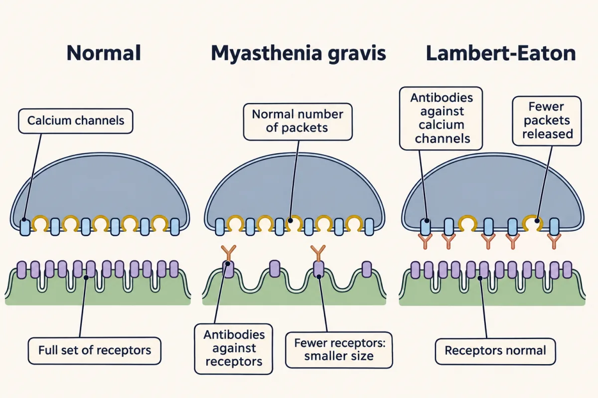
In myasthenia gravis, antibodies in most patients target the muscle’s acetylcholine receptors; others have antibodies against MuSK, a protein needed at the junction. Antibodies to the receptor can cross-link receptors and speed their removal, block them, or recruit complement that damages the postsynaptic membrane. Fewer receptors means a smaller q. Toyka and colleagues (1975) transferred an immunoglobulin fraction from patients’ serum into mice, which then had smaller miniatures and fewer junctional receptors (see the anecdote “A disease moved from patients to mice”).
Return to the worked example and cut q from 0.40 to 0.24 mV. Release also runs down during repeated impulses, as ready vesicles are used faster than they are replaced. For a clean illustration, treat each row as one impulse releasing a fixed number of packets, k: 60 on the first impulse, a quarter fewer (45) after run-down.
| Junction | packets on this impulse, k | size, q | count × size | balance point (steady-state illustration) | fires at 12 mV? |
|---|---|---|---|---|---|
| Normal, first impulse | 60 | 0.40 mV | 24.0 mV | 18.9 mV | yes |
| Normal, after run-down | 45 | 0.40 mV | 18.0 mV | 15.0 mV | yes |
| Myasthenic, first impulse | 60 | 0.24 mV | 14.4 mV | 12.4 mV | yes, barely |
| Myasthenic, after run-down | 45 | 0.24 mV | 10.8 mV | 9.6 mV | no |
| Lambert-Eaton, low count | 20 | 0.40 mV | 8.0 mV | 7.3 mV | no |
Only the myasthenic fibre fails after run-down. This is the fatigable weakness of myasthenia: muscles that work at first and weaken with use. Real counts fluctuate around their average, so a junction whose average sits just above threshold fails on some impulses even before run-down (Going deeper puts a number on it).
Acetylcholinesterase inhibitors act by letting each quantum’s acetylcholine last longer, so it survives long enough to reach more of the remaining receptors. That raises q partway back toward normal, the factor the disease lowered.
One caution. Poorly filled vesicles would also shrink q, so a small miniature does not by itself say which side is at fault. Pair the recording with a receptor count before you blame the receptors.
Lambert-Eaton syndrome: the count falls
In Lambert-Eaton syndrome the fault is presynaptic. Antibodies against the terminal’s voltage-gated calcium channels reduce calcium entry, so m is low while q is normal. An impulse releasing 20 packets of normal size gives about 7 to 8 mV, and the fibre fails.
Predict. Now stimulate a Lambert-Eaton junction rapidly, at 20 Hz. What happens to the count during the train, and why?
Check your prediction
The count rises. At 20 Hz the calcium left over from one impulse adds to the calcium of the next, so calcium builds up in the terminal. Because release rises steeply with calcium, a little extra calcium brings a large rise in m. During the train the response can climb back toward what the fibre needs. Slow repeated stimulation can instead give a decrement, a response that shrinks with each impulse: calcium clears between slow impulses, so run-down wins.
So the two diseases leave opposite fingerprints, provided resting potential, membrane properties and recording site are unchanged (if those shift, q shifts too):
| Recording | Points to |
|---|---|
| q down, m normal | the size side: receptors after the synapse, or vesicle filling before it |
| m down, q normal | the count side: release from the terminal |
Design problem
Two made-up muscle biopsies arrive for intracellular recording. In A, the miniature amplitude is reduced and the quantal content is normal. In B, the miniature amplitude is normal, the quantal content is low, and it rises during 20 Hz stimulation. Where is each defect, and what experiment would test your answer?
Saved in this browser only.
One way to do it
A is most likely postsynaptic: a smaller q with normal m fits fewer acetylcholine receptors, as in myasthenia gravis. To test whether a circulating factor is responsible, transfer the patient’s immunoglobulin fraction into mice and repeat the quantal analysis and a receptor count, as Toyka and colleagues did (1975, 1978). Predict smaller miniatures and fewer receptors, with m unchanged, as in their mice, or raised if the terminal compensates.
B is presynaptic: low m with normal q, rising during 20 Hz trains, fits reduced calcium entry, as in Lambert-Eaton syndrome. Test it by measuring m across a range of external calcium: if calcium entry is reduced, more calcium should raise release toward control levels, and you can compare the curve with control junctions. If an antibody is the cause, passive transfer of B’s immunoglobulins should lower m without changing q.
These are mechanisms for interpreting data, not clinical advice.
The contrast: a synapse with no packets
Not every synapse uses a transmitter. At an electrical synapse, channels called gap junctions join the two cells’ cytoplasm, and current passes directly with no transmitter step. There are no vesicles, so there is no quantal count or size and no release failures. The coupled response still has a size, and it can be too small to fire the next cell. Most electrical synapses are very fast and pass current both ways, which helps them synchronize cells. Some rectify, passing current more easily one way.
Next, transmitter systems asks where the brain’s other transmitters are made and cleared, and synaptic plasticity asks how release changes from one impulse to the next.
Going deeper
When the failure method goes wrong
The failure method follows from the count model only when p is small. Without the step-3 shortcut, the chance of a failure is exactly (1 − p)N, and −ln P(0) overestimates m. With m = 1, the error is 0.5% for N = 100 and p = 0.01, and 5% for N = 10 and p = 0.1. With m = 3, it is 19% for N = 10 and p = 0.3, and 39% for N = 6 and p = 0.5. So high release probability both makes failures vanish and biases the estimate upward.
Correcting for nonlinear summation
Write the endplate’s balance point with the resting membrane as one conductance G at Vrest and the packets as a total conductance g at the reversal potential Erev. One packet alone, small against G, moves Vm by q ≈ (gone / G) × DF, where DF = Erev − Vrest is the driving force at rest. Then k packets give
EPP = Vbalance − Vrest ≈ (k × q) / (1 + k × q / DF)
The tables use a fixed k. Real counts vary from impulse to impulse. Averaged over impulses the difference is small: for Poisson counts averaging 60 packets of 0.40 mV, the average of the formula is 18.90 mV, against 18.95 mV for exactly 60. But an average above threshold does not mean every impulse fires. With q = 0.24 mV this model needs at least 58 packets to reach 12 mV, and a Poisson count averaging 60 reaches that on only about 62% of impulses.
Inverting the formula gives v / (1 − v / DF) for a measured EPP v, the classical correction associated with Martin, which turns about 19 mV back into 24 mV. It assumes a steady state, and applied to brief EPPs it can overcorrect: McLachlan and Martin (1981) found this in their preparations and added an empirical factor. How well any such correction works depends on the response’s time course, the membrane and cable properties and where the electrode sits, so use one validated for the preparation.
Rectifying electrical synapses
Furshpan and Potter (1959) first showed rectification at the crayfish giant motor synapse. Shui and colleagues (2020) found that junctions built from the worm innexins UNC-7b and UNC-9, expressed in Xenopus oocytes, strongly favour current from the UNC-9 cell to the UNC-7b cell.
Central synapses depart from the frog picture
The count × size rule was built at the frog endplate. At central synapses a release site can release more than one vesicle, receptors can saturate, and q varies a lot from site to site. In cultured rat hippocampal boutons (small presynaptic terminals), Maschi and Klyachko (2020) saw two vesicles fuse at the same bouton after a single action potential (see the anecdote “Two vesicles from one bouton”).
Your notes
Select any text in the lesson to highlight it or add a note to it. Your highlights and notes are saved in this browser and collected in your notebook.
This browser is not letting the site save anything (a private window or strict privacy settings), so highlights and notes will be lost when you leave the page.
How we measure it
Intracellular recording at the endplate
A sharp glass microelectrode inside a muscle fibre near the nerve terminal records the endplate potential and the spontaneous miniatures. Their amplitudes, frequency and distance-dependence are the raw data of quantal analysis.
Quantal analysis
Compare evoked responses with miniatures under low release. Mean quantal content comes from the ratio of mean amplitudes or, under a Poisson model, from the failure rate; a change in quantal content usually points before the synapse, while a change in miniature size can come from receptors after it or from vesicle filling before it.
Electron microscopy with an extracellular tracer
Soak a stimulated terminal in horseradish peroxidase, fix it at timed points and find the tracer in internal membranes and vesicles. Where the tracer goes, and when, shows how vesicle membrane is retrieved and reused.
Passive transfer of patient antibodies
Inject an immunoglobulin fraction from patient serum into animals, then repeat the recordings and count receptors. If the disease signs transfer, a circulating factor is enough to cause them in that animal.
Practice questions on this lesson (3) → MCAT-style, original, each with an explanation
Where this lesson fits
Before thisReview first
- The Resting Membrane and Passive SignalsThis course · Lesson 3
You need the weighted-average balance point of conductances from there to follow how opening receptor channels depolarizes the endplate.
- The Action Potential and ConductionThis course · Lesson 4
The impulse that arrives at the terminal and opens calcium channels is described there, and this lesson starts from it.
After thisStudy next
- Transmitter Systems and DrugsThis course · Lesson 6
It takes the receptor and clearance steps here and asks how other transmitters and drugs change the size of a response.
- Synaptic PlasticityThis course · Lesson 8
It uses the count-times-size rule to ask whether changes in release come from the count or the size.
- Integration, Inhibition and NeuromodulationThis course · Lesson 7
It uses the postsynaptic conductance and balance-point idea to show how inhibition and summation shape the response.
Suggested by an AI model from the lessons themselves, then checked. How we use AI
Finish line
Test yourself
8 questions
Practice and MCAT-style, with explained answers.
Next · Lesson 6
Transmitter Systems and Drugs
Four drugs that act on GABA push inhibition in opposite directions. What decides which way a drug pushes?
Continue →