Ecology and Evolution · Unit 4: Interactions and communities
Predation and Community Effects
Rewritten on : new text, flashcards and film. Your notes and highlights stay, but the text around them may have moved.
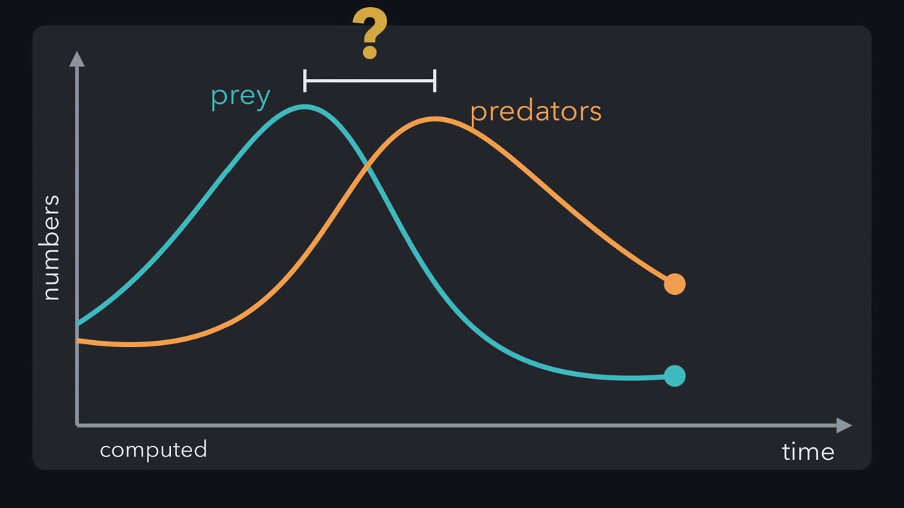
If predators eat prey, why do predator numbers keep climbing after the prey have started to fall?
Pause when the reading reaches a film, and offer to play it. Saved on this device.
Watch the film now, or keep listening
Builds on:Population Growth and RegulationCompetitionWhy these?
 ▶ Watch Two Ledgers, One Kill · 2:59
Read the transcript of “Two Ledgers, One Kill”
Film transcript: Two Ledgers, One Kill
If predators eat prey, why do predator numbers keep climbing after the prey have started to fall? The answer is in how one kill is counted. Every population keeps a ledger of births and deaths. Births push its numbers up, and deaths pull them down. Here are two ledgers, one for prey and one for predators. Now watch the kills. Each is a death in the prey's ledger. Each is also food, and on average, predators turn that food into births. So every kill is entered twice. That double entry ties the two ledgers together. The more predators there are, the faster each prey dies. The more prey there are, the faster predators breed. First ask when the prey stop changing.
Each prey's birth rate stays fixed, but its risk of death grows with every predator. At one predator number, P*, the two balance. Now ask when the predators stop changing. Each predator must eat enough prey to replace itself. That happens at one prey number, N*. With more prey, predators increase. With fewer, they decrease.
Put both thresholds on one picture, with prey across and predators up. The two lines cut it into four zones. Each zone has its own pair of directions. Start a dot in the bottom right, with many prey and few predators. Following the arrows, it circles the crossing point counter-clockwise, and returns to where it began. Stop the dot where the prey curve reaches its top. The prey have just peaked. Are the predators rising or falling?
Still rising. The prey are falling, but there are still more of them than N*. So each predator still eats more than it needs to replace itself. The predators peak only when the prey drop through N*. So the predator peak comes after the prey peak. Nothing in the model builds in a delay. The lag comes from the bookkeeping. Start the dot somewhere else, and it traces a different loop. In this classical model, each start with both populations present and away from the crossing point keeps its own loop. Where it starts sets the size of the cycle. So every kill, entered in both ledgers, ties them together. In this simple model, each population's per capita growth rate is set by the other's numbers.
From the film
- Each kill is a death for the prey and food that, on average, predators turn into births, so each population's per capita growth rate is set by the other's numbers.
- Prey increase while predators are fewer than P* = r/a; predators increase while prey are more than N* = m/(ea).
- Predators keep rising after prey have peaked, so predator peaks come after prey peaks, though the model builds in no delay.
- In the classical Lotka-Volterra model each start with both populations present and away from the equilibrium keeps its own closed loop, so the start sets the size of the cycle.
The first film followed kills into two ledgers, each population’s running account of births and deaths, and found the lag in that bookkeeping. This text starts from the equations it left out.
The one idea. Every kill is entered in two ledgers: a death in the prey’s, and food that, on average, the predators turn into births. So each population’s per capita (per individual) growth rate is set by the other’s numbers: r - aP for each prey, eaN - m for each predator. And a predator can affect species it rarely or never eats, even helping some it also eats, by changing the numbers or behaviour of the species in between.
Scope: the two rates belong to the classical Lotka-Volterra model below, and a population’s total change is its per capita rate times its own numbers. The reach to other species comes from field experiments, and its size and even its sign depend on the community.
Two ledgers, written as equations
In population growth each population changed by its own births and deaths. A predator is a consumer that kills and eats other organisms, its prey. Alfred Lotka (1925, in his book Elements of Physical Biology) and Vito Volterra (1926, in Nature) independently wrote the two ledgers as equations. With N prey and P predators:
dN/dt = rN - aNP dP/dt = eaNP - mP
Here r is the prey’s per capita growth rate without predators (per day). The attack rate a is the risk of being caught that one predator adds to each prey (units: per predator per day), so aP is each prey’s death rate from predation and aNP is the number of prey eaten per day. The conversion e is the average number of new predators made per prey eaten, and m is the predators’ per capita death rate (per day). The ledgers are linked by rates, not kill by kill: aNP prey deaths per day feed eaNP predator births per day. Divided by N and by P, the equations give the one idea’s per capita rates.
The assumptions are strong. Without predators the prey grow exponentially, with no carrying capacity. Without prey the predators decline exponentially. Each predator’s intake rises in proportion to prey numbers with no handling time (the time spent catching and eating each prey), so a predator never gets full. Populations are well mixed (every predator equally likely to meet every prey), with no age structure, no space and constant parameters.
The first film’s two threshold lines are isoclines: the sets of numbers at which one population stops changing. Set each per capita rate to zero: r - aP = 0 gives P = r/a, and eaN - m = 0 gives N = m/(ea). Where the two lines cross is the equilibrium:
N = m/(ea) P = r/a**
Predict. The prey start breeding twice as fast (r doubles) and nothing else changes. At the new balance point, which population is larger than before: the prey, the predators, or both?
Check your prediction
Only the predators. N* = m/(ea) contains no r, so the prey equilibrium does not move; P* = r/a doubles. With the worked numbers below, (500, 100) becomes (500, 200). Each equilibrium is set by the other population’s parameters: faster prey breeding feeds more predators, and the extra predators eat the extra prey.
Worked problem. These numbers are made up for illustration: r = 1 per day, a = 0.01 per predator per day, e = 0.1 predators per prey eaten, m = 0.5 per day. Today there are N = 400 prey and P = 50 predators.
- Prey rate. Prey births are rN = 1 x 400 = 400 prey per day. Prey eaten are aNP = 0.01 x 400 x 50 = 200 prey per day. So dN/dt = 400 - 200 = +200 prey per day.
- Predator rate. Predator production is eaNP = 0.1 x 200 = 20 predators per day. Predator deaths are mP = 0.5 x 50 = 25 predators per day. So dP/dt = 20 - 25 = -5 predators per day.
- Equilibrium. N* = 0.5 / (0.1 x 0.01) = 0.5 / 0.001 = 500 prey. P* = 1 / 0.01 = 100 predators. Check: at (500, 100), prey births are 500 and prey eaten are 0.01 x 500 x 100 = 500, so dN/dt = 0; predator production is 0.1 x 500 = 50 and deaths are 0.5 x 100 = 50, so dP/dt = 0.
- Read the state. Prey are below 500 and predators below 100: the bottom-left zone, where prey rise and predators fall. The simulation below starts here, at (400, 50); run it and note which curve turns first.
- prey isocline: P = r/a
- predator isocline: N = m/(ea)
- orbit through the start
- start
- equilibrium (N*, P*)
- Equilibrium N* = m/(ea)
- 500
- Equilibrium P* = r/a
- 100
- Period of this orbit, in this sketch (integrated from the equations)
- —
- Near-equilibrium period 2π/√(rm)
- —
- prey N
- predators P
- prey peak
- predator peak
Pick a start to see its orbit.
In this sketch: prey grow exponentially without predators (no self-limitation), each predator’s intake rises in proportion to prey numbers with no handling time, the populations are well mixed with no age structure, and r = 1 per day, a = 0.01 per predator per day and e = 0.1 predators per prey eaten stay fixed, and the model is continuous, so values below 1 are not real individuals. Units on the plot are individuals and days from the lesson’s illustration, not data on any real species.
The rule to keep: in the classical model every start sits on its own closed, neutral orbit, so the start sets the amplitude, and predators peak after prey.
What the classical cycle leaves out
With both populations present and away from the equilibrium, the loops are neutrally stable, like a marble on one of many nested, frictionless tracks: a nudge moves it to another track, and it circles that one instead, with no single cycle pulling it back.
Averaged over any full loop, the numbers equal N* and P*. Over one loop each population ends where it began, so its per capita rate averages zero, which requires the average of P to be r/a (and of N, m/(ea)). On the loop through (400, 50) that gives 500 prey and 100 predators, to within rounding.
Hence Volterra’s fishing argument: harvest both populations at the same per capita rate h, and the averages become (m + h)/(ea) prey and (r - h)/a predators, prey up and predators down, as long as h stays below r so that predators persist.
Predict. Give the worked-problem prey a carrying capacity, K = 400, so that without predators they settle at 400. Can the predators persist?
Check your prediction
No. Each predator replaces itself only when prey exceed N* = 500. Even at 400 prey, a rare predator’s per capita rate is eaN - m = 0.001 x 400 - 0.5 = -0.1 per day, so predators decline to extinction and the prey settle at 400.
Two changes to the assumptions matter most:
| Change to the model | What happens to the cycles |
|---|---|
| Prey self-limitation (logistic growth with carrying capacity K) | The neutral cycles disappear. If K is above N*, the populations settle at the equilibrium, often through damped oscillations, and the prey line tilts to P = (r/a)(1 - N/K), so the predator equilibrium falls below r/a: with the worked numbers and K = 2000, 100 x (1 - 500/2000) = 75 predators at 500 prey. If K is below N*, predators die out. |
| Handling time as well, so predators get full | For some parameter values the model settles onto one cycle whose size does not depend on the start (a limit cycle); for others it settles at an equilibrium, or the predators die out. |
Real records rarely fit the classical model either (Going deeper).
So far each kill has touched only two ledgers. But prey also compete with other species, so a predator can reach species it never eats. The second film follows that link on a rocky shore.
Read the transcript of “Fifteen to Eight”
Film transcript: Fifteen to Eight
The first film showed each kill entered in two ledgers. Now follow the kills one link further, to the species the prey compete with. You might expect every species a predator eats to do better without it. So what happens to a rocky shore when its sea star is gone? On this rocky shore, space on the rock is a limiting resource: its supply caps the populations that use it. Mussels are the strongest competitors for that space. The sea star Pisaster ochraceus eats mussels. It also eats barnacles, chitons, limpets and snails. Follow the orange arrows to each of its prey. In the early 1960s, Robert Paine began keeping Pisaster off one patch of shore at Mukkaw Bay, Washington.
He left a neighbouring stretch alone as a control, and surveyed both along line transects. The predator is gone from the patch. Will the number of species holding space on the rock go up, or down? Down. By his 1966 report, the removal patch held 8 species on the rock instead of 15. The control did not lose species in the same way. Here is how the patch filled. Acorn barnacles settled first and took most of the open rock. Then small mussels and gooseneck barnacles crowded them out. Algae lost their space. With Pisaster eating mussels, space kept opening for weaker competitors. Without it, mussels took the rock. The sea star raised richness by freeing space, not by eating species that harmed the rest.
Now look at one chiton. Pisaster eats chitons, so the sea star costs it some lives. But the sea star also keeps mussels off the rock, which keeps the chitons' space and food. Two arrows, with opposite signs. Without the sea star, chitons left the patch for lack of space and food. So here, the sea star's indirect help to some of its own prey outweighed what it ate. In a short note three years after his report, Paine used the word keystone. A keystone species has an effect on its community that is large relative to its abundance. Eating the dominant competitor, and so helping weaker ones, is called keystone predation. But this was one removal patch and one control.
It was a strong local result, not yet a general law. So a predator's effects can run through the species it eats, to the species they compete with. On Paine's shore, they did.
From the film
- Paine kept the sea star Pisaster ochraceus off one patch of shore at Mukkaw Bay, Washington, beside an untouched control.
- Without Pisaster, mussels, the strongest competitors for space on the rock, spread, and the species holding space on the rock fell from 15 to 8.
- Pisaster's effects ran through the mussels it ate to the species they compete with: it kept space open, including for some species it also ate.
- A keystone species has an effect on its community that is large relative to its abundance.
- This was one removal patch and one control: a strong local result, not yet a general law.
What one shore can and cannot show
The film’s count of 15 to 8 covered only species holding space on the rock. A mussel bed is itself a habitat: count the species living among the mussels and the result can reverse (Going deeper).
The keystone label compares effect with abundance, so the most common species is not a keystone by default: at Mukkaw Bay the mussels were the dominant competitor (the winner of the contest for space), and Pisaster was the keystone.
The chiton’s two arrows are the general case. A predator’s net effect on a species combines its direct effects (killing it, or changing how it behaves) with effects passed through other species, and the two can pull in opposite directions. Larger limpets left the patch as well as the chitons, so there the indirect help won. A weaker species gains only if release from the dominant competitor outweighs what the predator costs it directly, and heavier predation can reverse that balance. So a keystone predator can raise richness (the number of species), not always does. Why space on a rock is a limiting resource (one whose supply caps the populations that use it) is the subject of competition.
Cascades through killing and through fear
A trophic level is a feeding position in a food chain: plants, herbivores, carnivores. A trophic cascade is an indirect predator effect that extends through several trophic levels: predator to herbivore to plant.
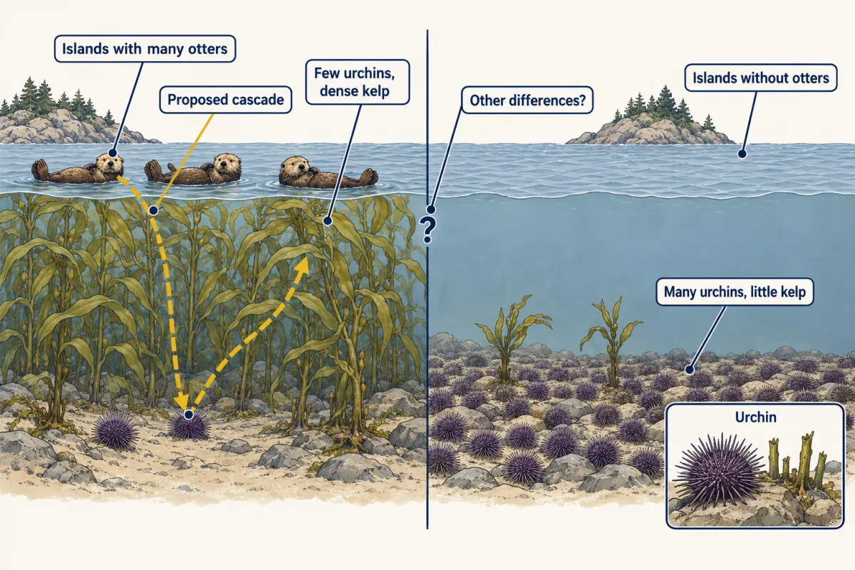
In a 1974 paper, James Estes and John Palmisano compared islands in the western Aleutians, Alaska: Amchitka, where a dense otter population had recovered after fur hunting, and Shemya, where otters had not come back (figure). Otters eat urchins, and urchins graze kelp, so the urchin and kelp pattern fits a two-link cascade, but no one removed otters. Later evidence came from a change over time: when sea otters declined across western Alaska in the 1990s, probably because killer whales ate more of them, urchins increased and kelp beds were lost.
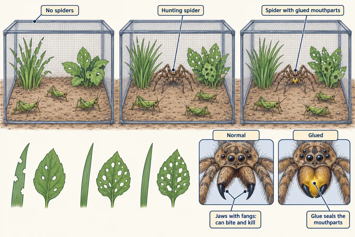
A density-mediated cascade works by killing herbivores, so fewer are left to eat plants. A trait-mediated cascade works by changing what surviving herbivores do, through the risk of being eaten: fear. In enclosures in a Connecticut old field, Andrew Beckerman, Maria Uriarte and Oswald Schmitz (1997) pulled them apart. They kept grasshoppers with no spiders, with hunting spiders, or with spiders whose mouthparts were glued so they could not kill.
Predict. Spiders that cannot kill: will the plants in their enclosures look like those with no spiders, or like those with hunting spiders?
Check your prediction
Like those with hunting spiders (figure below), because grasshoppers changed how long they fed and what they ate; the authors noted they may also have moved into the herbs for shelter. The authors traced the plant effect to risk rather than deaths, and not every plant benefited.
Landscape-scale cascades are harder to pin down. Wolves were reintroduced to Yellowstone National Park in the mid-1990s, and willow recovery has often been credited to them. In an experiment by Kristin Marshall, Thompson Hobbs and David Cooper (2013), reducing browsing alone did not bring the willows to the 2-metre height they used as their recovery criterion (design under Going deeper). Wolves were never an experimental treatment. A 2024 extension of the ten-year experiment to about two decades, and published disagreement over how willow recovery should be measured, leave the park-wide question open.
How far one system generalizes
Paine extended the removals himself: by 1974 he reported that after Pisaster was removed, mussels moved down the shore at both Mukkaw Bay and Tatoosh Island, with no change at control sites. A 2025 review by Anthony Gillis and colleagues found 25 publications that explicitly manipulated predators to test keystone predation: 10 reported consistent support, 7 found the effect context-dependent and 8 found none. Their search relied on the term itself, so it could miss studies that used other words, and a vote count is not an estimate of how often keystone predation occurs. So a keystone result on one shore is a hypothesis for the next shore, not a given.
Sea-star wasting disease, which killed Pisaster along much of the Pacific coast from 2013, has since run a coast-scale removal (Going deeper).
Design problem
Design a study that tests whether keystone predation by Pisaster generalizes across the coast. Say what you would measure, how you would replicate, and what result would count against generality.
Saved in this browser only.
One way to do it
Choose many sites that differ in wave exposure and mussel recruitment, since both could change how fast mussels take space. At each site assign several plots to removal or control at random. Survey every plot before removal and yearly for several years after (a before-after-control-impact design), to separate a change from what was already happening.
Fix the list of taxa you count before you start, so richness means the same thing everywhere. Measure mussel cover in every plot: if removal lowers richness, mussel cover should rise first, which tests the mechanism.
Use the sea-star wasting die-off from 2013 as a natural experiment, comparing shores that lost most of their Pisaster with shores that lost fewer; the die-off was not randomly assigned.
Expect context dependence. If richness falls where mussel recruitment is high and changes little where it is low, keystone predation is real but conditional, which fits the split in the Gillis review above.
Going deeper
Real data rarely fit the classical model
The famous hare and lynx cycle comes from fur-trade records, which reflect trapping effort as well as animal numbers. In the 1950s Carl Huffaker could keep predatory and plant-eating mites coexisting on oranges only when he made the arena patchy, a story taken up in movement and spatial populations. And rapid evolution of prey defenses can reshape cycles, as Takehito Yoshida and colleagues found with rotifers and algae, the subject of mutualism, parasitism and coevolution.
The period of the cycle
Near the equilibrium the cycle takes about 2 pi / square root of (rm) = 6.283 / square root of 0.5 = 6.283 / 0.707 = 8.89 days. This is a small-amplitude approximation. The larger orbit that passes through (400, 50) takes about 9.3 days, computed by solving the equations numerically.
How the patch filled, and when the word keystone appeared
In the film’s sequence, the acorn barnacles took most of the open rock within months. Kevin Lafferty and Thomas Suchanek pointed out in 2016 that mussel beds shelter over 300 associated species. Counting those, they argued, removing Pisaster would raise community-wide richness. The memorial to Paine in PNAS dates the keystone term to a short note he published in 1969. Keep the three dates apart: removal began in the early 1960s, the paper is from 1966, and the term is from 1969.
The Yellowstone experiment in detail
Marshall, Hobbs and Cooper ran a ten-year factorial experiment at four small-stream sites on the northern range, crossing fences that excluded browsers such as elk with simulated beaver dams, which raised July water tables by 33 cm on average.
What the wasting die-off showed
Monica Moritsch and Peter Raimondi (2018) found that sea-star counts at monitoring sites could recover while biomass, a proxy for predation potential, stayed below 40% of its pre-outbreak level in 2015 to 2017 at most sites outside North Central California, because recovering populations were made of small stars. Near Monterey, Joshua Smith and colleagues (2025) reported that mussels grew larger and spread lower on the shore after Pisaster collapsed, and they inferred that eating more mussels contributed in part to a local rise in sea otters.
Your notes
Select any text in the lesson to highlight it or add a note to it. Your highlights and notes are saved in this browser and collected in your notebook.
This browser is not letting the site save anything (a private window or strict privacy settings), so highlights and notes will be lost when you leave the page.
How we measure it
Predator removal with an adjacent control
Keep a predator out of one area and leave a neighboring area untouched, then survey both over time, for example along line transects. A difference that appears after removal points to the predator, but with one pair of plots it says nothing about how widely the effect holds.
Risk-only predator manipulation
Disable the predator's ability to kill, here by gluing a spider's mouthparts, while leaving it present to be sensed. Comparing risk-only, normal-predator and no-predator treatments separates effects carried by killing from effects carried by prey behavior.
Comparison of sites with and without a predator
Survey prey and plants at places where a predator is present and places where it is absent, as Estes and Palmisano did on Aleutian islands. It is quick and large in scale, but the places may differ in other ways, so it supports a cascade without proving one.
Factorial exclosure experiment
Cross two treatments, such as fencing out browsers and building simulated beaver dams, so every combination is present at each site. This lets you estimate each factor's effect and whether one matters only when the other is present.
Practice questions on this lesson (3) → MCAT-style, original, each with an explanation
Where this lesson fits
Before thisReview first
- Population Growth and RegulationThis course · Lesson 14
The prey's exponential growth rate r and the idea of per capita rates come from there.
- CompetitionThis course · Lesson 16
Paine's result depends on mussels outcompeting other species for space on the rock.
After thisStudy next
- Mutualism, Parasitism and CoevolutionThis course · Lesson 18
It reads the predator-prey phase lag in real data and shows how evolving prey defences reshape cycles.
- Diversity, Disturbance and SuccessionThis course · Lesson 19
A keystone predator changes how many species coexist, which this lesson measures with richness and disturbance.
- Energy Flow and ProductivityThis course · Lesson 21
It takes trophic levels further by tracking how much energy passes from plants to herbivores to predators.
Elsewhere on the siteFilms, simulations and method films in other courses
- Island of wolves and mooseSimulation · Life Science
The island wolf and moose model lets you watch predator and prey numbers rise and fall together.
- Follow the Energy ArrowsFilm · Life Science
It shows how effects of eating pass along food-web arrows, a basis for trophic cascades.
Suggested by an AI model from the lessons themselves, then checked. How we use AI
Finish line
Test yourself
8 questions
Practice and MCAT-style, with explained answers.
Next · Lesson 18
Mutualism, Parasitism and Coevolution
The same root fungus can help a plant in poor soil and cost it in rich soil. Is it a mutualist or a parasite?
Continue →