Genetics and Molecular Biology · Unit 1: Inheritance
New to this? Review it at high school level: Beyond Dominant and Recessive
Reading Pedigrees: Human Inheritance
Rewritten on : new text, flashcards and film. Your notes and highlights stay, but the text around them may have moved.
Your brother has cystic fibrosis and you do not. Is your chance of being a carrier 1/2 or 2/3?
Pause when the reading reaches a film, and offer to play it. Saved on this device.
Watch the film now, or keep listening
Builds on:Mendel's Peas: Segregation and Independent AssortmentProbability, Crosses and the Chi-Square TestExtending Mendel: Dominance, Multiple Alleles and Gene InteractionWhy these?
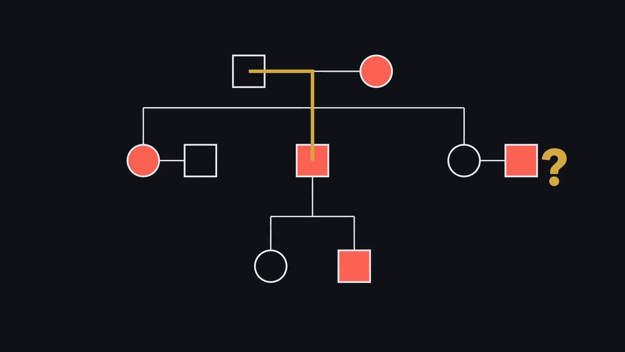 ▶ Watch The Pedigree as a Model Test · 3:36
Read the transcript of “The Pedigree as a Model Test”
Film transcript: The Pedigree as a Model Test
Can one family observation eliminate an inheritance model? Watch this pedigree become a test instead of a pattern to memorize. The answer depends on what each model says should be possible. This is why a pedigree works like a model test.
A pedigree records people, relationships, and a named phenotype. Shapes identify family members, connecting lines show relationships, and fill marks affected people. Always read its key. The same symbol can mean something different when the chart defines it differently. Now place a model over the chart. Each inheritance model predicts where an allele can travel and which relatives can receive it. The chart becomes evidence because every line now makes a claim. An autosomal route can move through either parent and either sex. A dominant model lets an affected heterozygous parent pass the allele to children of either sex. An affected child of two unaffected parents contradicts that simple dominant model.
A recessive allele can hide in unaffected carriers. It may appear among siblings when each parent contributes a recessive allele. Here, unaffected parents can carry the allele without showing the trait. Sex-linked models restrict the route. A father gives his X chromosome to daughters and his Y chromosome to sons. That route makes sex and parental origin informative, not merely decorative. An affected father also has an affected son. Could an X-linked allele have travelled directly from that father to that son? Follow the chromosome route before you answer.
No. The son's X chromosome came from his mother. Demonstrated father-to-son transmission therefore contradicts both X-linked models under these assumptions. An affected pair alone shows it only if the mother carries no copy. Mitochondrial inheritance draws a different route. Mothers can transmit mitochondrial DNA to children, while fathers normally transmit none. This maternal route differs from mitochondrial diseases caused by nuclear genes. Fitting predictions support a model; one contradiction can rule it out.
Compatibility adds support, but an observation the model forbids carries sharper information. The model earns confidence by surviving such tests. That is the guiding rule for this simple-model test. That test has a scope. It assumes full penetrance, no new mutation, correct relationships, and the simple model being tested. Change an assumption, and a seeming contradiction may need another explanation. A fitting chart supports a model without proving it. Other models or hidden biology may predict the same small family. Small families often lack the relative who would distinguish those models.
From the film
- Fitting predictions support a model; one contradiction can rule it out.
- A pedigree records phenotypes and relationships; its key defines the symbols.
- Each simple inheritance model predicts who can transmit an allele to whom.
- The exclusion tests assume full penetrance, no new mutation and correct relationships.
Human geneticists cannot set up crosses, so they work backwards from existing families. A pedigree is a family tree drawn to a shared code.
The one idea. Fitting predictions support a model; one contradiction can rule it out.
Scope: the five simple, single-gene models used here, assuming full penetrance (everyone with the genotype shows the trait), no new mutation and correct family relationships. A model that fits is supported, not proved.
Read the evidence first
The first film used three symbols; the full code has more. In the 2022 revision of the National Society of Genetic Counselors standard, a square is a man or boy, a circle is a woman or girl, and a diamond is a nonbinary person or someone whose sex or gender is not specified. The revision ties shape to gender and records sex assigned at birth separately. A filled symbol means affected by the condition named in the key; a diagonal slash marks someone who has died.
A horizontal line joins partners. A vertical line drops to a horizontal sibship line, from which each child hangs. A double partner line marks consanguinity: the partners are related by descent, as first cousins are. Roman numerals label generations, and people are numbered left to right, so II-3 identifies one person. An arrow marks the proband, through whom the family came to attention.
A carrier is heterozygous for a recessive allele and usually does not show the trait. Many textbook charts put a central dot in the circle of a woman known to carry an X-linked recessive allele. The 2022 revision shows carrier status differently; check the key.
Predict. Two partners are joined by a double line. Can you conclude that both carry the allele being studied?
Check your prediction
No. The line records shared ancestry, not genotype. Consanguinity raises the chance that both carry the same rare allele but does not establish carrier status or prove recessive inheritance.
Test five inheritance models
| Model | Prediction under the simple model | A contradiction |
|---|---|---|
| Autosomal dominant | One copy in a heterozygote is enough. The trait usually appears in successive generations and both sexes; father-to-son transmission is possible. An affected heterozygote and unaffected partner give each child a 1/2 allele risk. | An affected child has two unaffected parents. |
| Autosomal recessive | Affected people have two pathogenic alleles at one locus, identical or different. Unaffected carrier parents can have affected children of either sex, so cases often cluster among siblings, with few affected relatives elsewhere. Shared ancestry is more common because relatives are likelier to carry the same rare allele. | Two affected parents have an unaffected child, if the same gene causes both parents’ trait. |
| X-linked recessive | A male has one X, so one copy can affect him. Affected men are much more common than affected women. An affected man passes the allele through carrier daughters to half their sons. Heterozygous women can show signs, partly through X-inactivation. | Demonstrated father-to-son transmission. An affected father-son pair establishes this only if the mother carries no copy. |
| X-linked dominant | An affected father passes the allele to every daughter and no son. An affected heterozygous mother passes it to half her children of either sex. | An affected father has an unaffected daughter or transmits the allele to a son. |
| Mitochondrial | Human mitochondrial DNA normally comes from the mother. An affected mother can have affected children of both sexes; an affected father transmits the trait to none. | Transmission from an affected father. |
Recessive deafness shows why that row’s qualification matters: different genes can cause deafness, so two deaf parents can have a hearing child. Mitochondrial DNA encodes only a handful of respiratory-chain subunits (see oxidative phosphorylation); most mitochondrial proteins are nuclear-encoded, so many mitochondrial diseases instead follow Mendelian patterns.
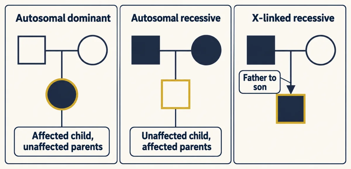
Predict. An affected father has an unaffected daughter. Under the scope above, which of the five models does that one observation rule out?
Check your prediction
Only X-linked dominant, because every daughter receives her father’s X. The other four models all allow an unaffected daughter.
Do not use “skips a generation” as proof of recessive inheritance; reduced penetrance can make a dominant allele appear to skip. Rett syndrome and fragile X syndrome, introduced in synapse disorders, are X-linked examples complicated by new mutations and repeat expansion.
Once a model survives those tests, the next question is how strongly each possible genotype is supported.
Read the transcript of “Evidence Reweights the Possibilities”
Film transcript: Evidence Reweights the Possibilities
The first film tested inheritance models against family observations. How can learning that someone is unaffected raise their carrier probability? The surprise comes from comparing only genotypes still compatible with the observation.
Begin with every genotype the inheritance model allows. Give each possibility its starting weight before using the person's phenotype. These weights come from transmission rules and any population assumptions. Write them down before looking at the answer you hope to get. Now condition on what you observed. Any genotype incompatible with that observation loses its weight. Compatible possibilities remain. This is a filter, not a change to the person's cells. Keep the survivors in their original proportions. Suppose a new observation excludes one visible possibility. Which tiles should remain in the probability bar, and what must happen next? Watch the total bar, not just the disappearing tile.
Remove the incompatible tile. Then stretch the survivors to fill the whole bar again. That second step is renormalizing. The surviving possibilities now divide all the probability between them. A carrier tile can therefore occupy more of the remaining bar. This can happen even when the person is unaffected. The comparison set became smaller. Nothing happened to the person's DNA.
Evidence changes genotype probabilities, not genotypes. Only the description of your uncertainty changed. Sometimes evidence does not eliminate a hypothesis. It is merely more likely under one hypothesis than another. Bayes' rule handles that case. The observation changes weights without making either hypothesis impossible. Likelihood measures that predictive fit. Each hypothesis starts with a prior weight. Multiply that weight by how well the hypothesis predicts the observation. A better prediction earns a larger updated weight. A weak prediction earns less. Finally, renormalize those weighted hypotheses. Their new shares form the posterior: the probabilities after accounting for the evidence. Together, those shares still fill the complete probability bar.
More observations repeat the same cycle. Start with current weights, ask what each hypothesis predicts, apply the evidence, then renormalize. Each new fact becomes the next filter. The method remains the same. The answer still depends on the model. Penetrance, new mutation, family relationships, and population assumptions all shape those starting weights and likelihoods. If an assumption changes, recompute instead of reusing the old answer. With that picture, the text can calculate exact carrier and recurrence probabilities. Keep the filter, the weights, and the assumptions visible. The worked examples begin with different family evidence.
From the film
- Evidence changes genotype probabilities, not genotypes.
- Conditioning removes incompatible outcomes and renormalizes the outcomes that remain.
- Bayes' rule weights each hypothesis by how well it predicts the evidence.
- Risk calculations are only as sound as their stated inheritance assumptions.
Conditional probability: the 2/3 rule
The second film reweighted schematic tiles; now put exact numbers on them. A woman’s brother has cystic fibrosis, an autosomal recessive disorder caused by two pathogenic cystic fibrosis transmembrane conductance regulator (CFTR) alleles. Her parents and she are unaffected. Her partner has no family history. What is the probability that their first child is affected?
Within the scope above, assume a partner carrier frequency of 1/25, a figure often quoted for northern European ancestry and lower in many populations; it is an exercise assumption, not a universal number.
Her affected brother shows that both parents are carriers, Aa. Before her phenotype is used, Aa x Aa gives four equally likely outcomes: AA, Aa (A from the mother), aA (A from the father) and aa, each 1/4.
Predict. She is unaffected. Which outcome disappears, and what fraction of the remaining outcomes are carriers?
Check your prediction
The affected aa outcome disappears. Of the three equal outcomes left, Aa and aA are carriers:
P(carrier | unaffected) = (1/2) / (1/4 + 1/2) = (1/2) / (3/4) = 2/3
If both partners are carriers (her partner with probability 1/25), both pass the recessive allele with probability 1/4. Therefore
P(affected child) = 2/3 x 1/25 x 1/4 = 2/300 = 1/150
As a decimal check, 1/150 is about 0.0067, and 0.667 x 0.04 x 0.25 = 0.0067. The tempting 1/2 was her carrier probability before her unaffected phenotype removed one outcome. These are logic exercises, not risk figures for a real family.
Condition on what you know: knowing a sibling is unaffected removes one outcome and shrinks the denominator. These numbers assume full penetrance, no new mutation, correct relationships and a carrier frequency of 1/25; they are exercises in the logic, not risk figures for a real family.
Updating with evidence: Bayes and unaffected sons
Here evidence reweights the hypotheses instead of deleting one, so Bayes’ rule from the second film applies. A woman’s mother is a known carrier of a fully penetrant X-linked recessive allele, and her father is unaffected. The untested woman has two unaffected sons.
Her unaffected father gave her a normal X and her mother one of two X chromosomes, so her prior is 1/2 carrier and 1/2 not carrier.
Predict. Are two unaffected sons more likely if she is a carrier or if she is not? Should her carrier probability rise or fall?
Check your prediction
They are more likely if she is not a carrier, so her carrier probability falls. If she is a carrier, each son is unaffected with probability 1/2, so the likelihood for two is 1/4. If she is not a carrier, the likelihood is 1.
Multiply each prior (the weight before the evidence) by its likelihood (the chance of the evidence under that hypothesis): carrier gives 1/2 x 1/4 = 1/8; not carrier gives 1/2 x 1 = 1/2. Normalize the two weights:
P(carrier | two unaffected sons) = (1/8) / (1/8 + 1/2) = 1/5
Prior odds of 1 : 1 become posterior odds of 1 : 4, because the evidence is four times likelier if she is not a carrier. Under the same model, her next son’s affected risk is 1/5 x 1/2 = 1/10.
Why real pedigrees mislead
One contradiction rules a model out only inside the scope, and real families break the scope in four ways.
- Genotype may not predict one visible phenotype. Huntington disease is dominant, but symptoms usually begin in adulthood, so a young unaffected child of an affected parent may carry the allele. Penetrance also depends on CAG repeat length in HTT: about 36 to 39 repeats is usually described as reduced penetrance, and 40 or more as full penetrance. Variable expressivity means the same genotype produces different clinical pictures.
- A variant may be new or mosaic. A new pathogenic variant can produce a dominant disorder in a child of unaffected parents, which looks exactly like the observation that rules out autosomal dominant inheritance. In germline mosaicism, a parent carries a variant in only some cells, including some sperm or eggs. In a study of 58 families with one affected child and an apparently new variant, deep sequencing of several parental tissues estimated recurrence below 0.1% in 35 families; 5 had parental mosaicism associated with higher risk, and three fathers had the variant in 5.6 to 12.1% of sperm DNA.
- Mitochondrial genotype can be a mixture. With heteroplasmy, a cell contains normal and mutant mitochondrial DNA. A mother can transmit different proportions to different children, so severity varies and some children may be unaffected.
- A family may be too small to reveal the pattern.
Predict. If two carrier parents have only two children, is seeing no affected child surprising enough to reject autosomal recessive inheritance?
Check your prediction
No. Each child has a 3/4 chance to be unaffected, so the chance that both are unaffected is (3/4)2 = 9/16, more than half the time. Small families can look as though nothing is inherited.
Apparent exceptions also need molecular checks: among 11,035 trios, all seven apparent paternal mitochondrial signals were explained by a mitochondrial-derived nuclear insert shared by father and child.
Design problem
An affected woman has five children, all affected. Her affected son has three children, none affected. Her affected daughter has two children, both affected. Severity varies. Decide between mitochondrial and X-linked dominant inheritance, and identify data that would settle it.
Saved in this browser only.
One way to do it
Test the affected son. He transmits no mitochondrial DNA, so three unaffected children fit mitochondrial inheritance. Under fully penetrant X-linked dominant inheritance every daughter receives his affected X, so they exclude that model only if at least one is a daughter.
The rest does not discriminate. Both models fit an affected mother with affected children. A mother transmits mitochondria to every child; under X-linked dominant inheritance, five affected children of a heterozygous mother has probability (1/2)5 = 1/32: possible but unlikely.
Variable severity fits both models, so it cannot decide between them. Under heteroplasmy children receive different mutant fractions; X-inactivation in women can vary an X-linked dominant phenotype.
Settle it molecularly. An affected father with an affected daughter whose mother lies outside the maternal line and lacks the family’s mitochondrial variant would exclude mitochondrial inheritance. Or sequence affected and unaffected relatives, seek a mitochondrial variant confined to the maternal line, and measure heteroplasmy in several tissues. Heteroplasmy tracking severity, with the variant absent from the son’s children, would support the mitochondrial model.
Your notes
Select any text in the lesson to highlight it or add a note to it. Your highlights and notes are saved in this browser and collected in your notebook.
This browser is not letting the site save anything (a private window or strict privacy settings), so highlights and notes will be lost when you leave the page.
How we measure it
Pedigree construction with standardized nomenclature
A family history is drawn with agreed symbols for sex or gender, affection status, relationships, deceased members and the proband. A shared code lets any reader test an inheritance model against the same chart.
Conditional and Bayesian risk calculation
Genotype probabilities are enumerated under a stated model, then conditioned on what is observed, such as an unaffected phenotype or a set of unaffected children. The result is a probability for an untested person under those assumptions.
Linkage analysis with DNA markers
A variable DNA marker is typed in as many family members as possible and tested for co-inheritance with the disease. A marker that travels with the disease far more often than chance places the gene near it, as for Huntington disease on chromosome 4.
Deep sequencing of several tissues
A variant is sequenced to very high depth in blood, saliva, sperm or other tissues of each parent. The fraction of reads carrying it estimates the level of mosaicism or heteroplasmy in each tissue, which a single blood test can miss.
Practice questions on this lesson (5) → MCAT-style, original, each with an explanation
Where this lesson fits
Before thisReview first
- Mendel's Peas: Segregation and Independent AssortmentThis course · Lesson 1
You need segregation and the 1/4 outcomes of a cross between carriers to build the carrier and recurrence calculations.
- Probability, Crosses and the Chi-Square TestThis course · Lesson 3
The 2/3 rule and the Bayes update rest on the product and sum rules for crosses taught there.
- Extending Mendel: Dominance, Multiple Alleles and Gene InteractionThis course · Lesson 4
Penetrance and the dominance patterns used to test each model are introduced there.
After thisStudy next
- Sex Linkage, Dosage Compensation and Non-Mendelian InheritanceThis course · Lesson 6
It explains the X-linked and non-Mendelian transmission patterns that this lesson only uses as pedigree signatures.
- Chromosome Number and Structure: Aneuploidy and RearrangementsThis course · Lesson 7
Aneuploidy and rearrangements show another reason a pedigree can mislead when the trait is not a simple single-gene one.
- Population Genetics: Hardy-Weinberg and Evolutionary ForcesThis course · Lesson 25
Carrier frequencies like the 1/25 assumed here come from allele frequencies and Hardy-Weinberg.
Elsewhere on the siteFilms, simulations and method films in other courses
- Where Can White Flowers Hide?Film · Life Science
It shows how recessive alleles hide in parents and pass on, the basis of carrier risk.
- Cross and countSimulation · Biology
It lets you cross carrier parents and count outcomes, giving the 1/4 and 3/4 chances used for pedigrees.
- What Can Cross a Generation?Film · Life Science
It separates gene-coded traits that pass through sex cells from changes gained in life, which pedigrees must distinguish.
Suggested by an AI model from the lessons themselves, then checked. How we use AI
Finish line
Test yourself
10 questions
Practice and MCAT-style, with explained answers.
Next · Lesson 6
Sex Linkage, Dosage Compensation and Non-Mendelian Inheritance
Why can swapping which parent has white eyes change every son?
Continue →← Lesson 4 · Extending Mendel: Dominance, Multiple Alleles and Gene Interaction