Genetics and Molecular Biology · Unit 2: Mapping and gene function
Linkage and Recombination Mapping
Rewritten on : new text, flashcards and film. Your notes and highlights stay, but the text around them may have moved.
Independent assortment predicts four equal test-cross classes. Why do two classes dominate?
Pause when the reading reaches a film, and offer to play it. Saved on this device.
Watch the film now, or keep listening
Builds on:Mendel's Peas: Segregation and Independent AssortmentChromosomes and Meiosis: The Physical Basis of Mendel's LawsProbability, Crosses and the Chi-Square TestWhy these?
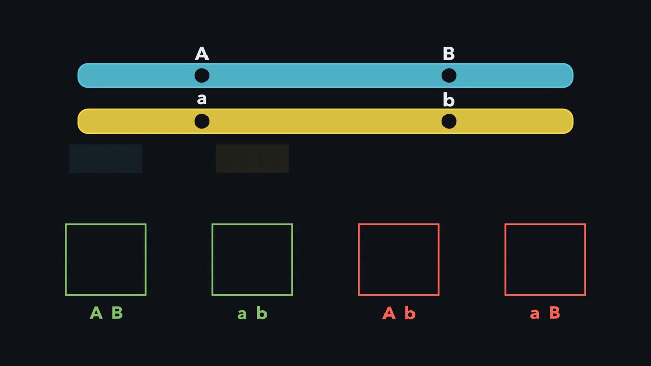 ▶ Watch When Four Classes Refuse to Be Equal · 3:41
Read the transcript of “When Four Classes Refuse to Be Equal”
Film transcript: When Four Classes Refuse to Be Equal
Why do two test-cross classes overwhelm the other two? A blue chromosome and a gold partner pair in meiosis. Each carries the same marker positions. Their allele combinations begin intact, yet the offspring bins grow unevenly. The puzzle is what those bins reveal about gametes.
With scorable traits, a test cross makes one parent's gametes visible. The heterozygote can contribute big A big B or big A little b. It can also contribute little a big B or little a little b. The tester always contributes recessive alleles. Each offspring therefore carries a readable copy of the heterozygote's gamete. Independent assortment would feed every bin equally. Instead, the inherited combinations repeatedly fill two bins faster. That excess is the signature of linkage in this cross.
Linked means the loci share a chromosome closely enough for their association to appear in the scored progeny. First read the chromosomes the heterozygote received. Big A with big B is one inherited combination. Little a with little b is the other. Those are parental, even before counting offspring. The mixed combinations are recombinant. This inherited arrangement is phase. Class size can support that assignment, but phase defines it. Each homologue has already copied itself, so four chromatids lie side by side. A crossover joins matching positions on non-sister chromatids. When the exchange falls between the markers, the right-hand segments trade places.
Two chromatids keep their inherited combinations. The exchanged chromatids carry new combinations, which feed the recombinant bins. Now slide the right marker farther away while crossover positions keep appearing along the chromatids. Which pair of bins should claim a larger share over a short interval? Hold the chromosome picture in your mind.
The recombinant pair grows. A wider interval offers more places for a crossover to land between the markers. Over a short interval, a second crossover between the markers is rare, so few exchanges stay hidden. The recombinant share can therefore serve as an estimate of genetic map distance. Add both recombinant classes before dividing by all offspring. Write the result as a percentage. For a short interval, that percentage estimates centimorgans on the genetic map. It does not measure a fixed length of DNA.
Different chromosome regions and different sexes can convert physical spacing differently. The workflow is now stable. Read the parents. Name the parental and recombinant classes from phase. Add the recombinant classes, then divide by the total. Only then use the short-interval ruler. The next question is what happens when crossovers can hide one another.
From the film
- For short intervals, recombination frequency estimates map distance.
- A test cross makes the double heterozygote's four gamete classes visible in its offspring.
- Phase, not class size, defines which combinations are parental and recombinant.
- A crossover between two loci can separate their alleles into new combinations.
Test-cross fruit flies that carry two mutations and score 1,000 offspring. Mendel’s law of independent assortment predicts that 500 will show one grandparent’s combination of traits or the other’s. You count 830.
Independent assortment (Mendel’s peas, probability and crosses) holds for loci on different chromosomes. For loci close together on one chromosome it fails, and the failure becomes a ruler.
The one idea. For short intervals, recombination frequency estimates map distance; over long intervals, hidden crossovers make it underestimate distance.
Scope: this is two-locus mapping when progeny accurately report gametes. “Short” means double crossovers in the interval are rare. Phase identifies recombinants first, and distance is genetic rather than physical.
Read the four classes before counting them
A locus is a gene’s place on a chromosome; its versions are alleles. Take two loci, A and B, with recessive alleles a and b. The first film showed how a test cross, a double heterozygote mated to an a b / a b tester, makes each offspring’s phenotype name the heterozygote’s gamete. Unlinked loci give the four classes 1:1:1:1; when the inherited combinations come back more often, the loci are linked, near each other on one chromosome.
The combinations inherited by the heterozygote are the parental classes. The other two are recombinant. Which is which depends on phase, the arrangement of alleles in that heterozygote:
- Coupling (cis), A B / a b: the dominant alleles came in on one chromosome. Parental classes are A B and a b.
- Repulsion (trans), A b / a B: each chromosome carries one dominant allele. Parental classes are A b and a B.
Predict. A female received A b from her mother and a B from her father. Before seeing any offspring, which two test-cross classes are parental?
Check your prediction
A b and a B are parental because those are the combinations she received; A B and a b are recombinant. Parental classes are usually larger, but inheritance defines them, not their counts.
Crossing over makes recombinants
In prophase I, each chromosome has already copied itself into two sister chromatids, and the partner chromosomes, or homologues, pair, placing four chromatids side by side (see chromosomes and meiosis). Crossing over is a reciprocal exchange of matching segments between non-sister chromatids, one from each homologue. The cross-shaped contact that remains visible is a chiasma.
In the first film’s single crossover, the two chromatids that took part became A b and a B and the other two stayed parental. Because the exchange is reciprocal, the two recombinant classes should be about equal in a test cross, as should the two parental classes. A large difference within a pair suggests that one genotype survives less well.
Predict. In one reciprocal pair you count 85 A b offspring but only 20 a B offspring. What should you question before treating the total as an unbiased crossover count?
Check your prediction
Question equal survival and scoring. A reciprocal exchange makes the two recombinant combinations about equally, so a strong deficit in one class can mean that genotype survives poorly or is hard to score.
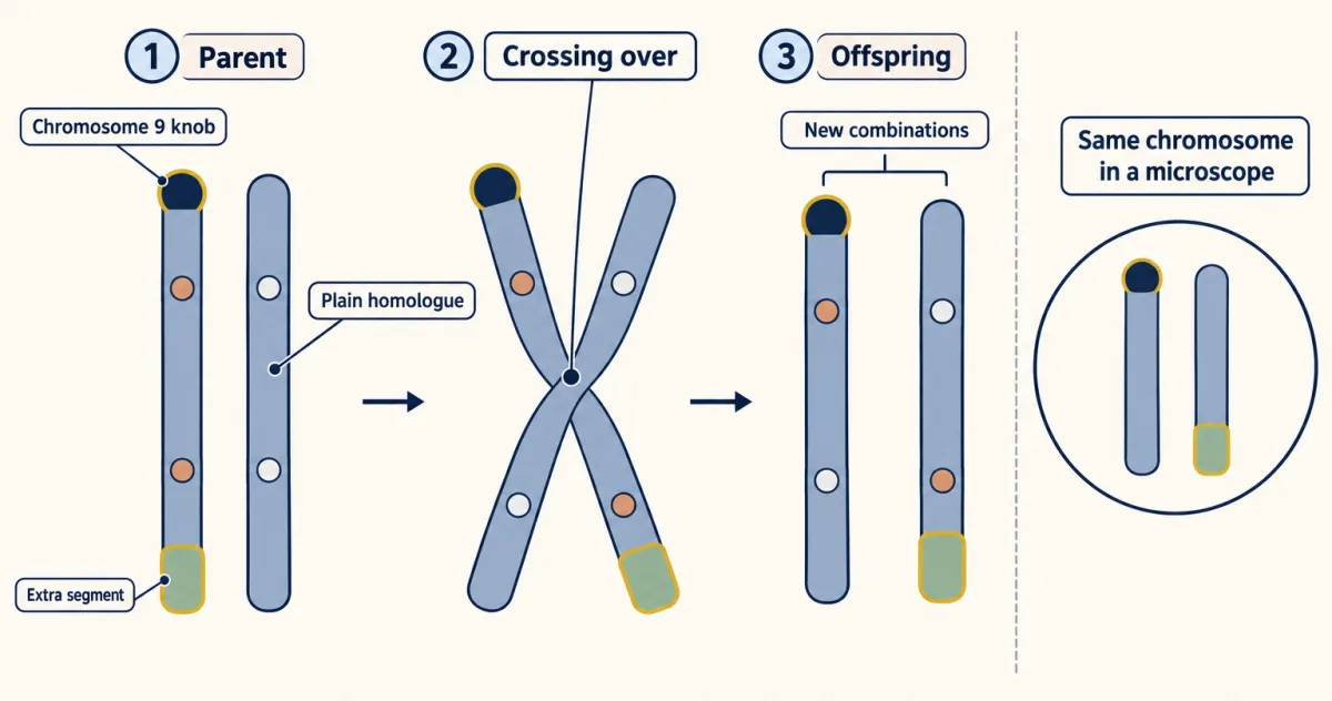
Was crossing over a physical swap? In 1931 Harriet Creighton and Barbara McClintock used maize whose two copies of chromosome 9 looked different. One copy had a visible knob at one end and an extra segment from another chromosome at the other; its partner had neither, so offspring could be classified by both genes and chromosome structure.
Predict. If a new gene combination comes from physical exchange, what should happen to the visible knob and extra segment?
Check your prediction
The landmarks should appear in new combinations too. That is what Creighton and McClintock found: recombinant genes travelled with the chromosome structures predicted by an exchange. Curt Stern reported the same correlation in Drosophila that year, using X chromosomes with visible structural changes.
How DNA strands are broken and rejoined is covered in DNA repair and recombination.
Sturtevant’s map: frequency as distance
The first film turned the recombinant share into a ruler; here is the same step as an equation. Recombination frequency (RF) is the number of recombinant progeny divided by the total number scored.
In words The map distance in centimorgans is a hundred times the recombination frequency, and the recombination frequency is the recombinant offspring divided by all the offspring.
- cM“centimorgans”
- map distance between the two loci. Use this conversion for short intervals only.
- RF“R F, recombination frequency”
- the fraction of offspring in the recombinant classes, between 0 and 0.5
Sanity check If no offspring are recombinant, RF = 0 and the loci map to the same spot. RF cannot rise past 0.5, so a test cross never reads more than 50 cM directly; the section on the 50% ceiling explains why.
Try one number
Round numbers to keep the arithmetic easy (not from a real cross): 50 recombinant flies out of 500.
RF = 50 / 500 = 0.10, or 10%. Map distance = 100 × 0.10 = 10 cM.
Need a refresher? rates and “per”
One map unit, or centimorgan (cM), named for Morgan, corresponds to 1% recombinant progeny over a short interval. It is not a length of DNA: the ratio of DNA to centimorgans varies along chromosomes, among species and between sexes, and crossover rates also vary among individuals, so a map is an estimate for a stated population and sex. Drosophila melanogaster males normally make no crossover gametes; in humans and many other species the two sexes also give different maps.
Worked problem. Assume complete penetrance, equal survival of all classes, and accurate scoring. A Drosophila female heterozygous for recessive mutations a and b on one autosome received A B from one parent and a b from the other, so she is in coupling. She is test-crossed to an a b / a b male. Of 1,000 progeny:
| Class | Count |
|---|---|
| A B | 420 |
| a b | 410 |
| A b | 85 |
| a B | 85 |
- Name the classes from the phase. She received A B and a b, so those are parental: 420 + 410 = 830. A b and a B are recombinant: 85 + 85 = 170. Here they are also the smallest classes, as expected for linked loci.
- Calculate RF. RF = 170 / 1,000 = 0.17, or 17%. Read directly, the map distance is about 17 cM.
- Test for linkage with the chi-square score from probability and crosses. Independent assortment predicts 250 in each class. Chi-square = (420 - 250)2/250 + (410 - 250)2/250 + 2 × (85 - 250)2/250 = 115.6 + 102.4 + 108.9 + 108.9 = 435.8, with 3 degrees of freedom. The 5% critical value from a chi-square table is 7.81. The excess of parentals is far beyond chance.
- Predict the other phase. A female carrying the same loci in repulsion, A b / a B, would still give 17% recombinants, but now A B and a b are the recombinant classes: 8.5% each (half of 17%), with 41.5% each of A b and a B (half of the remaining 83%).
Step 4 is where students slip: “recombinants are the two smallest classes” is a habit, not a rule. It fails when you must predict the classes before any flies hatch, and it fails when a class survives poorly enough to shrink below a recombinant class.
An RF of 17% gives an uncorrected estimate of 17 cM. Whether that interval is short enough for RF to approximate distance depends on how often multiple crossovers occur; over long intervals, hidden crossovers make recombination frequency underestimate distance. The second film shows how.
Read the transcript of “Why the Map Outgrows the Count”
Film transcript: Why the Map Outgrows the Count
The first film turned recombinant offspring into a short chromosome ruler. Why does that ruler fail when the interval grows? Reuse the blue and gold homologues. Move their outside markers apart, and let more crossover sparks fall between them. The map keeps growing, but the observed count cannot follow forever.
A two-point cross does not count crossover events. It reads only the final combination of the outside markers. One exchange between them flips a parental combination into a recombinant one. Another exchange can flip that combination again. The gamete remembers its ending, not the number of turns. The chromatid now looks recombinant at the outside markers. What will those markers show after another crossover lands inside the same interval? Follow only their colours, not the crossed segments in the middle.
The second flip can restore the parental outside combination. The middle still records exchanged material, but a two-point score misses it. Even numbers of effective flips look parental. Odd numbers look recombinant. Long intervals contain more hidden histories that finish with the same visible answer. Across many meioses, repeated flips make parental and recombinant endings equally likely. Recombination frequency therefore approaches its ceiling. So distant linked loci can look unlinked, like loci on different chromosomes. A two-point result at the ceiling cannot distinguish those cases. Now plot what the count can see against map distance. Use Haldane's no-interference equation, not a sketch.
The computed curve starts close to a straight line, then bends toward the ceiling. Distance continues across the axis while the observable frequency loses sensitivity. A third marker breaks a long span into shorter intervals. Count each short interval where fewer exchanges stay hidden. Place those distances end to end on one chromosome. Their map distances add. Their raw recombination frequencies do not, because the whole-span count can erase double crossovers. The computed curve is a model, not a universal correction. Haldane assumes independent crossover placement. Interference changes how often nearby crossovers occur, so another function may fit better. The durable practice is to map short intervals, add their distances, and state the model behind any correction.
The count reports a final marker state. The map represents the expected number of crossovers per chromatid across the interval. Those quantities track closely only while hidden exchanges are rare. As the interval grows, the map can keep lengthening after the count has nearly stopped changing.
From the film
- Over long intervals, hidden crossovers make recombination frequency underestimate distance.
- A two-point count records the final allele combination, not the number of crossovers.
- Recombination frequency approaches 50%, so distant linked loci can look unlinked.
- Map distances add across short intervals; raw recombination frequencies do not.
The 50% ceiling, and what a mapping function corrects
The second film showed that a two-point count reads only the final outside-marker combination on each scored chromatid, so an even number of exchanges affecting that chromatid hides. (An even number of crossovers in the whole bivalent need not hide, because different crossovers can involve different chromatids.) Why the average stops at exactly one half, the film did not show; the reason is the four chromatids. A crossover between the loci involves two of them, so a meiosis with one crossover in the interval gives half recombinant products. A second crossover between the same loci either recombines them again or puts them back, depending on which chromatids it joins; on average the recombinant share stays at one half. Loci far apart on one chromosome therefore give about 50%, the same as loci on different chromosomes. A two-point cross cannot tell those apart; linkage of both loci to a third marker can.
Map distance is the expected number of crossovers per chromatid in an interval, measured in morgans (1 morgan = 100 cM); recombination frequency is the fraction of gametes whose two marker alleles finish in a recombinant combination. In 1919 J. B. S. Haldane gave a mapping function that connects the two, assuming crossovers form independently along the chromosome. The second film plotted its curve; here is the equation.
In words The recombination frequency is one half of one minus e to the minus two d.
- RF“R F”
- the recombination frequency you would observe in a test cross
- e−2d“e to the minus two d”
- under Haldane's assumption, the chance that a meiosis has no crossover at all between the two loci. e is about 2.718.
- d“d”
- the true map distance in morgans (1 morgan = 100 cM)
Sanity check At d = 0, e0 = 1 and RF = 0: loci in the same place never recombine. As d grows, e−2d shrinks toward 0 and RF climbs toward 1/2, the 50% ceiling. For small d, RF is close to d, which is why short intervals can be read directly.
Try one number
A 50 cM interval is d = 0.5 morgans, so 2d = 1.
e−1 is about 0.368 (see e and ln). 1 − 0.368 = 0.632, and half of that is 0.316.
So a 50 cM interval gives only about 31.6% recombinants: read directly, it would look like 31.6 cM.
Where it comes from optional
Optional: where it comes from. A distance of d morgans means d crossovers per chromatid on average, so 2d per meiosis, because each crossover involves two of the four chromatids. If crossovers fall at random, the chance that a meiosis has none in the interval is e−2d. A meiosis with at least one crossover gives, on average, half recombinant products, as the four-chromatid argument above showed. So RF = 1/2 × (1 − e−2d).
Need a refresher? e and ln · powers and roots
To get a distance from an observed RF under this model, rearrange:
- Multiply both sides by 2: 2 RF = 1 − e−2d.
- Swap terms: e−2d = 1 − 2 RF.
- Take the natural log of both sides (ln undoes e): −2d = ln(1 − 2 RF).
- Divide by −2: d = −1/2 × ln(1 − 2 RF).
For the worked cross, Haldane’s model asks what distance would produce an RF of 0.17 if crossovers occurred independently:
d = −1/2 × ln(1 − 0.34) = −1/2 × ln(0.66) = 0.208 morgans (ln(0.66) is about −0.416, from a calculator’s ln key), or about 20.8 cM.
The gap grows with distance. Two adjacent intervals of 20 and 40 cM add to 60 cM, yet under the same model their own frequencies, 16.5% and 27.5%, would add to 44%, while the whole 60 cM span gives 34.9%.
- Recombinants (A b + a B)
- 0
- Observed RF
- 0
- Expected RF at this distance
- 0
- Distance read as 100 x RF (short-interval rule)
- 0
Recombination frequency tracks map distance only over short intervals; it climbs toward, and never passes, 50%, so long distances are underestimated. This is a sketch of the logic: the curve assumes crossovers form independently (Haldane), and real crossovers interfere, so it can overcorrect. Assumes equal survival of all classes and accurate scoring; a Drosophila female heterozygote.
Predict. If crossover interference makes nearby double crossovers rarer than Haldane assumes, will Haldane’s function tend to undercorrect or overcorrect an observed RF?
Check your prediction
It can overcorrect. Fewer double crossovers are hidden than the no-interference model expects, so less extra distance is needed. Kosambi’s function builds interference in and gives about 17.7 cM for the worked RF, closer to the direct 17 cM than Haldane’s 20.8 cM. Drosophila crossovers interfere strongly over short intervals, so for this cross the direct 17 cM is likely nearer the truth.
In most organisms studied, crossovers interfere: one makes another nearby less likely. Sturtevant suspected this, and single-sperm sequencing of 20 human donors detected it in every donor in 2020. No mapping function fits every organism, so the second film’s closing practice holds: map with short intervals and add them, and use a third marker to catch double crossovers, as in three-point mapping.
Design problem
You isolate a new recessive mutation in Drosophila, dumpy-like (dl), and suspect it lies on chromosome 2 near a known recessive marker, m. Design crosses to test whether dl and m are linked and to estimate the distance between them. Say what result would leave you unable to decide.
Saved in this browser only.
One way to do it
Build a heterozygote in known phase. Cross dl/dl flies to m/m flies. Every F1 fly is dl + / + m (+ is the wild-type allele), in repulsion, and you know the phase because you made it.
Use females. Because Drosophila melanogaster males normally make no crossover gametes, an F1 male gives only parental classes if dl and m share a chromosome, whatever the distance, and all four classes if they do not. A male test cross can show linkage but cannot measure distance. Test-cross F1 females to dl m / dl m males. If no double-mutant stock exists yet, you first recover a dl m recombinant chromosome from the progeny of F1 females.
Score enough flies. Score all four classes in several hundred progeny at least, more if the loci may be close, since a short interval yields few recombinants.
Test linkage without being fooled by survival. Check each locus alone for 1:1 (dl versus +, m versus +); a deficit of dumpy-like flies, for instance, would distort the four classes even if the loci were unlinked. Then test the association in a 2 x 2 table (dl versus + against m versus +) with a one-degree-of-freedom chi-square, which unequal survival at one locus does not inflate.
Calculate. Here the recombinants are wild type and dl m. RF = (wild type + dl m) / total, and the distance in cM is 100 x RF, corrected with a mapping function if RF is large.
Know the limit. An RF near 50% cannot tell a distant locus on chromosome 2 from one on another chromosome. To place dl, add a third marker on chromosome 2 and do a three-point cross, which also orders the three genes.
Going deeper
From coupling to a chromosome map
In 1905 William Bateson, Edith Saunders and Reginald Punnett reported that in the second generation of a sweet-pea cross, purple flowers went with long pollen, and red flowers with round pollen, far too often for independent assortment. They called this coupling and later explained it by gamete formation, not shared chromosomes.
In 1911 Thomas Hunt Morgan, whose laboratory found X-linked Drosophila mutants (see sex linkage), proposed the chromosome explanation. He drew on F. A. Janssens’s 1909 interpretation of crossed meiotic figures as chromosome exchanges.
As an undergraduate in Morgan’s laboratory, Alfred Sturtevant used crossover progeny as a distance index. His 1913 map placed six X-linked factors on one line and added short intervals. He warned that genetic and physical spacing need not match.
The mismatch that exposed hidden crossovers
Sturtevant’s short intervals placed B and M 57.6 units apart; a direct cross gave 37.6% recombinants. He proposed, as probable rather than proved, that double crossovers restored the parental outside markers.
Your notes
Select any text in the lesson to highlight it or add a note to it. Your highlights and notes are saved in this browser and collected in your notebook.
This browser is not letting the site save anything (a private window or strict privacy settings), so highlights and notes will be lost when you leave the page.
How we measure it
Two-point test cross
An organism heterozygous at two loci is crossed to one homozygous recessive at both. Each offspring's phenotype then reads directly which combination of alleles came in the heterozygote's gamete, so counting the classes counts parental and recombinant gametes.
Cytological chromosome markers
Partner chromosomes are made to look different, with a knob, a translocated piece or a broken arm, and offspring are classified both genetically and under the microscope. If gene recombination always comes with a visible exchange of landmarks, crossing over is physical.
Chi-square test against 1:1:1:1
Observed test-cross counts are compared with the counts expected if the loci assort independently. A large chi-square says the departure is unlikely to be chance; a separate test of each locus for 1:1 checks whether one allele survives less well.
Practice questions on this lesson (5) → MCAT-style, original, each with an explanation
Where this lesson fits
Before thisReview first
- Mendel's Peas: Segregation and Independent AssortmentThis course · Lesson 1
You need independent assortment and the 1:1:1:1 test-cross ratio from there, since linkage is a failure of that rule.
- Chromosomes and Meiosis: The Physical Basis of Mendel's LawsThis course · Lesson 2
You need homologue pairing, chromatids and chiasmata from there to see how crossing over makes recombinant gametes.
- Probability, Crosses and the Chi-Square TestThis course · Lesson 3
The chi-square test from there is used here to show the excess of parental classes is not chance.
After thisStudy next
- Three-Point Crosses: Gene Order and Double CrossoversThis course · Lesson 9
A third marker catches the double crossovers that a two-point count hides, putting genes in order.
- Bacterial and Phage Genetics: Conjugation, Transduction and TransformationThis course · Lesson 11
Mapping by timing or co-transfer extends the idea of distance from recombination to organisms without meiosis.
- Complementation and Gene Function: From Beadle and Tatum to BenzerThis course · Lesson 10
Once mutations are placed on the map, complementation tests whether they hit the same gene.
Elsewhere on the siteFilms, simulations and method films in other courses
- Homologs First, Sister Chromatids SecondFilm · Biology
It shows how meiosis shuffles chromosomes, including crossing over that makes recombinant gametes.
Suggested by an AI model from the lessons themselves, then checked. How we use AI
Finish line
Test yourself
10 questions
Practice and MCAT-style, with explained answers.
Next · Lesson 9
Three-Point Crosses: Gene Order and Double Crossovers
If two crossovers restore the outer genes' parental arrangement, how can offspring counts reveal them?
Continue →← Lesson 7 · Chromosome Number and Structure: Aneuploidy and Rearrangements