Ecology and Evolution · Unit 4: Interactions and communities
New to this? Review it at high school level: Succession in Virginia
Diversity, Disturbance and Succession
Rewritten on : new text, flashcards and film. Your notes and highlights stay, but the text around them may have moved.
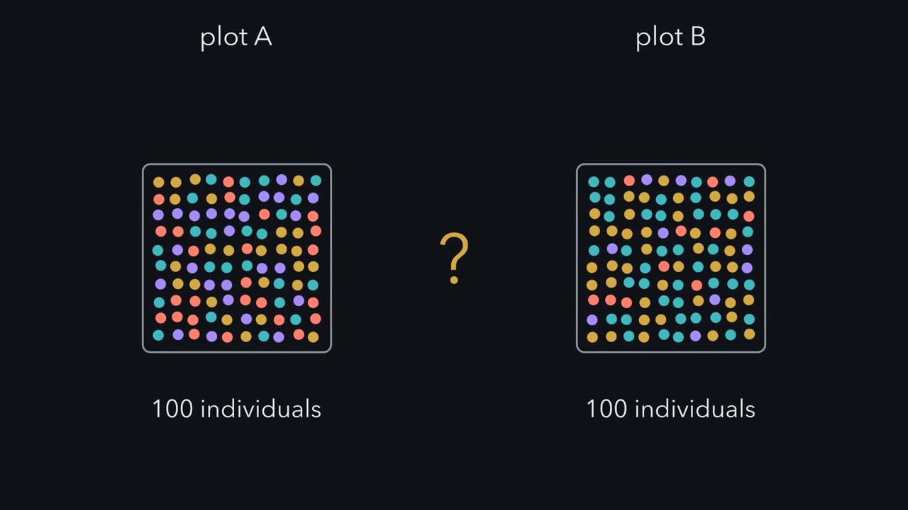
Two plots hold the same four species. Can one be more diverse than the other?
Pause when the reading reaches a film, and offer to play it. Saved on this device.
Watch the film now, or keep listening
Builds on:CompetitionPredation and Community EffectsWhy these?
 ▶ Watch How Many Species Is It Worth? · 3:11
Read the transcript of “How Many Species Is It Worth?”
Film transcript: How Many Species Is It Worth?
Two plots hold the same four species, a hundred individuals each. Can one be more diverse than the other? Count the species, and they tie. Look at the dots, and they do not look alike. Richness is the number of species present. Both plots have four, so richness calls it a tie. But richness counts every species once, however rare it is. It ignores abundance entirely. Diversity also asks how evenly the individuals are shared. In plot A, every species holds the same share. In plot B, two species hold most of the individuals, and two are rare. Here is a way to put richness and evenness on one scale.
Imagine a community in which every species is equally common. How many such species would score the same as plot B? That count is the effective number of species. For plot A, the answer is four, the same as its richness. For plot B, it is fewer than four, because two species hold most of the individuals. The measure has a dial, called the order. At order zero, every species counts once, however rare. As the order rises, common species count for more, and rare ones for less. Turn the dial for plot B. Its row of equal species shrinks, step by step, as its two rare species count for less. Plot A does not move, because nothing in it is rare. So the order you choose changes the number.
At order zero, the effective number is just the richness, so plot B ties plot A. Above order zero, it equals the richness only when every species is equally common. Always say which order you used. Now swap plot B's colours, so the rare species become the common ones. Nothing changes. These indices use only counts, never names, so none of them sees which species are present. One last test. A storm sweeps through plot B and kills the same share of every species. Most individuals die. What happens to its effective number?
Nothing happens to it. The counts drop, but every species keeps the same share. So the effective number stays exactly where it was. So a disturbance can change diversity in only two ways. It can change which species are present. Or it can change how evenly the individuals are shared, as the survivors regrow. Whether that raises or lowers diversity is a question for experiments.
From the film
- Richness counts species; diversity also asks how evenly the individuals are shared among them.
- An effective number of species is how many equally common species would give the same diversity value.
- At order zero it is the richness; above order zero it equals the richness only when every species is equally common, and it falls as a few species take over.
- These count-based indices use only counts, never names, so none of them sees which species are present: name the measure, its order and what it misses.
- A disturbance that kills the same share of every species leaves the shares, and so the effective number, unchanged; diversity changes only if who is present or how evenly they are shared changes.
The first film scored two plots as effective numbers of species. Here is where those numbers come from, and then how a community (the set of species living and interacting in one place) rebuilds after a disturbance.
The guiding idea. Any of the diversity indices here can be turned into an effective number of species: how many equally common species would give the same value. At order 0 it is simply the richness (the number of species present). Above order 0 it equals the richness only when every species is equally common, and it falls as a few species take over. These indices use only counts, never names, so succession and disturbance can change them only by changing which species are present or how evenly individuals are shared among them.
Scope: this holds for the count-based measures in this lesson (richness, Shannon, Simpson and their effective numbers); a similarity index that compares species lists, like the one in the forest study below, does see identity. The idea does not say whether disturbance raises or lowers diversity: that depends on how often it strikes, how hard, and in which system, and settling it needs a manipulation.
Counting a community: richness, evenness and effective species
Start with a species-by-count table: how many individuals of each species were counted. Richness, S, is the number of species present. Relative abundance, pi, is the proportion of individuals that belong to species i. Evenness describes how equally the individuals are spread among species.
Two indices combine richness and evenness. Shannon entropy, H, measures the uncertainty about which species the next individual you pick belongs to: zero if there is one species, larger as species are many and evenly spread. With the natural logarithm, as here, its unit is the nat. Simpson concentration, lambda, is the probability that two individuals drawn at random (with replacement) belong to the same species.
H = -sum of (pi x ln pi) lambda = sum of pi^2
Worked problem. The first film’s two plots, counted completely, 100 individuals each: sample A has 25, 25, 25 and 25; sample B has 40, 40, 10 and 10. Both have S = 4.
- Shannon entropy. In A every pi = 0.25, so HA = -4 x (0.25 x ln 0.25) = ln 4 = 1.386 nats. In B, 0.4 x ln 0.4 = -0.3665 and 0.1 x ln 0.1 = -0.2303, so HB = 2(0.3665) + 2(0.2303) = 0.733 + 0.461 = 1.194 nats.
- Simpson. λA = 4 x 0.252 = 0.25. λB = 2(0.16) + 2(0.01) = 0.34. The complements are 0.75 and 0.66.
- Back to species. exp H undoes the logarithm and turns nats into species: 4.00 for A, 3.30 for B. 1/lambda turns a matching probability into species: 4.00 for A, 2.94 for B. Simpson’s evenness E = (1/lambda)/S is 1.00 for A and 2.94/4 = 0.735 for B.
- Read it. “Simpson index” can mean lambda, 1 - lambda (the Gini-Simpson index, the probability that two draws differ) or 1/lambda. Reported as “Simpson index”, A = 0.25 and B = 0.34 make B look more diverse, though a larger lambda means less diversity. Name the convention.
The order, q, is the first film’s dial: as it rises from 0, rare species count for less, and at q = 2 for much less. Effective numbers of each order are called Hill numbers.
effective species: order 0 = S order 1 = exp H order 2 = 1/lambda
Why convert? Ten equally common species give a Gini-Simpson index of 0.90; twenty give 0.95. The community doubled and the index barely moved; the effective numbers read 10 and 20.
Predict. Plot C has five species, counted 60, 10, 10, 10 and 10 out of 100. Plot D has four, at 30, 30, 20 and 20. Which plot is more diverse?
Check your prediction
It depends on the order. C wins on richness, 5 species against 4. D wins at order 1 (3.92 effective species against 3.41) and order 2 (3.85 against 2.50): once abundance counts, C’s dominant species outweighs its extra rare ones. Name the order (Going deeper has a pair that swaps rank between orders 1 and 2).
- Richness S
- 4
- Shannon H (nats)
- 1.386
- Simpson λ
- 0.25
- Gini-Simpson 1 − λ
- 0.75
- exp H (species)
- 4.00
- 1/λ (species)
- 4.00
- Evenness E = (1/λ)/S
- 1.000
- Individuals counted
- 100
In this sketch: every individual is counted (complete counts, no sampling error), four labelled species, H uses the natural logarithm, and "Simpson" here means λ = Σ p² with 1 − λ and 1/λ named separately.
Rule to keep: richness ignores abundance, higher orders discount rare species, and no index tells you which species are present, so shuffling the labels changes nothing.
Observed richness also rises with sampling effort, since more individuals means more chances to find a rare species. Standardize before comparing, for example by rarefaction, which recalculates each sample at a common number of individuals.
Succession: three ways one community replaces another
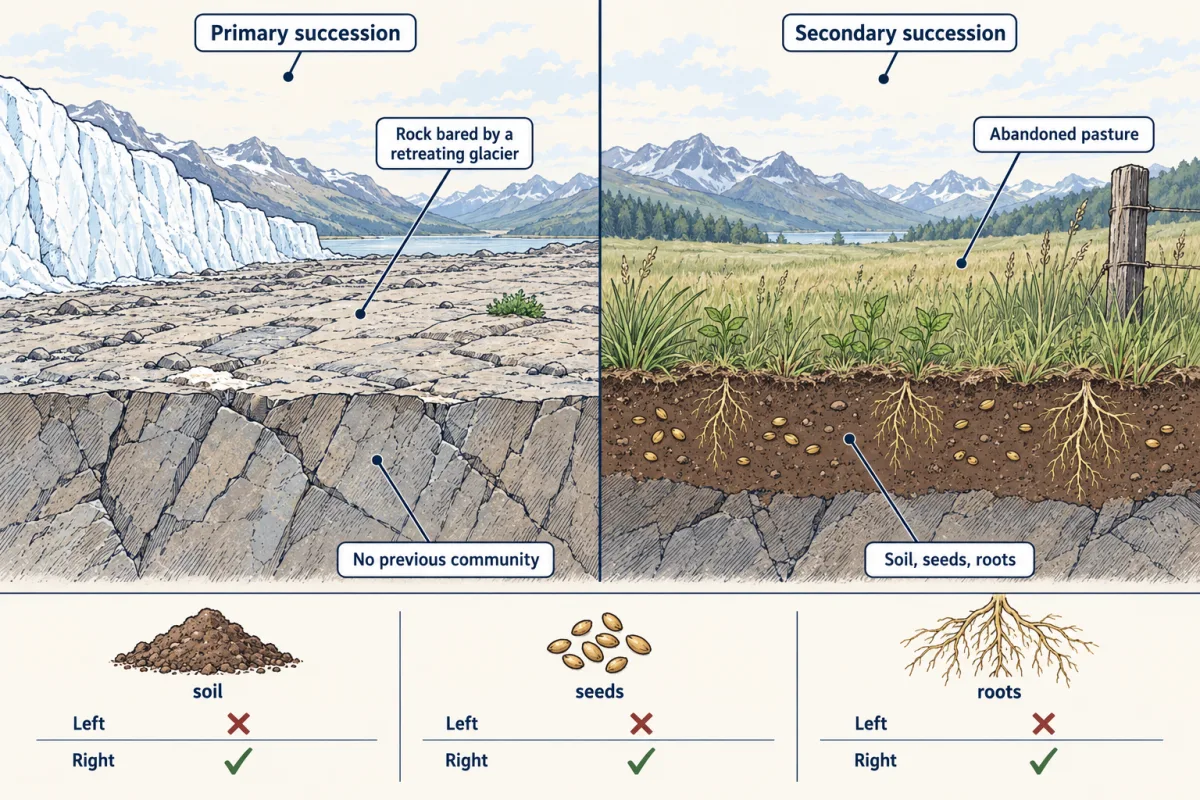
Succession is the change in species composition at a site over time after a disturbance, an event that kills or removes organisms and frees space or resources. Primary succession starts with no previous community: new lava, rock bared by a retreating glacier, a new seawall. Secondary succession follows a disturbance that leaves soil, seeds or roots behind: an abandoned pasture, a burned forest.
Microbes take part too: adding nitrogen and phosphorus together to young glacier soils shifted their bacteria toward those of much older soils, in one forefield (Going deeper).
Why does one set of species replace another? Joseph Connell and Ralph Slatyer (1977) set out three alternative models.
- Facilitation: early species change the site (adding soil, shade or nitrogen), and later species can establish only after that change.
- Tolerance: early species neither help nor much hinder later ones; later species persist because they can grow at lower resource levels.
- Inhibition: whoever arrives first holds the space and keeps later colonists out until it is damaged or dies.
All three produce early species followed by later ones, so watching the sequence cannot tell them apart. Removing the early occupants can.
Predict. Clear the early colonists from a plot as they settle. Under each model, do later species establish sooner, later, or about as soon as in untouched plots?
Check your prediction
| Model | What the early species do | Remove them, and later species establish… |
|---|---|---|
| Facilitation | change the site so later species can establish | later (delayed) |
| Tolerance | neither help nor much hinder | about as soon (little change) |
| Inhibition | hold the space | sooner |
Real results are often mixed: early colonists can help some later species and hinder others, and tolerance is hard to tell from inhibition in the field, so a removal result usually tests particular species, not one model for a whole site. The same logic runs removal experiments in competition and predation.
Nothing in these models has a goal: early species alter conditions, and later species do better or worse as a result. Nor does succession necessarily run to one fixed endpoint: where it goes depends on which species arrive, in what order, and how often the site is disturbed again.
Many succession studies use a chronosequence, a set of sites of different ages read as one trajectory (a space-for-time substitution). In Neotropical secondary forests read this way, richness recovered much more than species composition (Rozendaal and colleagues, 2019; numbers in Going deeper): the count can look recovered while the species are still different.
All three models describe interactions that unfold between disturbances. Repeated disturbance can interrupt or redirect succession, and the second film follows that on a boulder shore.
Read the transcript of “Holding a Boulder Still”
Film transcript: Holding a Boulder Still
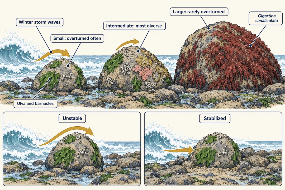
Succession needs time, but on a rocky shore, winter waves keep turning boulders over. Middle-sized boulders hold the most diverse communities. Is that because of their size, or because of how often waves turn them? Wayne Sousa studied a boulder field on the southern California coast.
There, winter storm waves overturn the boulders. Overturning a boulder kills some or all of the algae on its upper face, and opens space. So each turn sets succession on that surface back. Picture a clock on each upper face, counting time since it was last cleared. On a fully cleared face, Ulva and barnacles usually settled first. Red algae followed. Without another overturning, Gigartina often came to dominate. Survivors can change that order. Small boulders are overturned often, so their clocks keep snapping back. They carry sparse early communities of Ulva and barnacles.
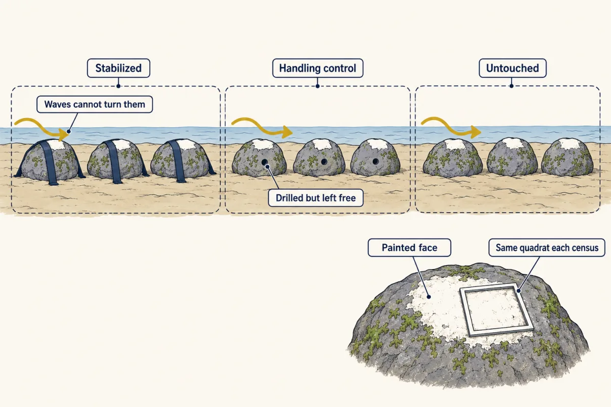
Large boulders rarely turn, and Gigartina takes them over. Boulders of intermediate size turn now and then. They are caught partway along, and they carry the most diverse communities. But size and overturning travel together. The small rocks are the ones that flip. A bigger surface might simply hold more species, so the pattern alone cannot say which matters. So Sousa held some small boulders still, fixed in place so waves could not turn them. Similar small boulders were left loose nearby, free to roll. Both sets sat at the same height on the shore. If size is what matters, the fixed small boulders should stay sparse. If overturning is what matters, what should they become?
They moved on. Ulva gave way, and red algae, Gigartina among them, came to cover most of the fixed rocks. The loose rocks kept their early communities. The fixed small boulders became as species-rich and diverse as larger, intermediate-sized boulders. Their smaller surface did not stop them. On that shore, how often rocks overturned, not surface area alone, accounted for the pattern. This test varied one thing, how often a patch is reset. It did not vary how hard each event hits, and it holds for one shore. Even there, the season of a census mattered. In spring, large boulders were no longer poorer in species.
So disturbance sets succession back, and how often it strikes helps decide how far a patch gets.
From the film
- On Sousa's southern California shore, winter waves overturned small boulders often and large ones rarely, and intermediate boulders carried the most diverse communities.
- Each overturning kills some or all of the algae on the upper face and sets succession on that surface back; how often it strikes helps decide how far a patch gets.
- Boulder size and how often a boulder is overturned travelled together, so the pattern alone could not say which mattered.
- Small boulders fixed so waves could not turn them were taken over by later red algae and became as species-rich and diverse as larger, intermediate-sized boulders, while loose ones stayed early.
- The test varied how often disturbance struck, not how hard, and it holds for one shore.
Disturbance: Sousa’s boulders and the debate over the hump
The second film did not name the hypothesis its boulders tested. The intermediate disturbance hypothesis (IDH) predicts that the diversity of competing species peaks at intermediate disturbance frequency or intensity: too little disturbance, and the best competitors exclude the rest; too much, and only fast colonizers survive. Connell’s 1978 paper in Science on tropical forests and coral reefs is usually cited, though J. Philip Grime (1973) and others gave earlier versions; Sousa’s (1979) boulders are a classic test of it.
Frequency and intensity together
Sousa varied how often a patch is reset. A disturbance also has an intensity: the share of organisms each event kills. Alex Hall and colleagues (2012) crossed five frequencies with three intensities, from 10% to 99.999% of cells killed per event, in microcosms (small unshaken laboratory cultures) of the bacterium Pseudomonas fluorescens. It quickly evolves several morphotypes (heritable colony forms), so the community is variants of one strain, not separate species.
Predict. Hold intensity fixed and vary frequency. Will diversity against frequency have the same shape at all three intensities?
Check your prediction
No. At 10% mortality, frequency made no difference to diversity. At 99.9%, diversity was greatest at intermediate and high frequencies. At 99.999%, it peaked clearly at an intermediate frequency. Read the other way, diversity rose with intensity when disturbances were rare but peaked at an intermediate intensity when they were frequent. Frequency and intensity interact, so a study that varies only one of them gives an incomplete answer: it holds at the level of the factor it kept fixed.
The experiment measured outcomes, not mechanisms: diversity might move through the types that regrow fastest after each hit, or through rare types lost by chance when few cells survive, but neither was tested. Gibbons and colleagues (2016) added time: in a lake-water bacterial community, a diversity peak appeared only briefly, while community states mixed (“A peak that did not last”).
Is the hypothesis right? Jeremy Fox (2013) argued it should be abandoned: its usual mechanisms are logically flawed, and humped curves are found only rarely. Michael Huston (2014) replied that critics had ignored the linked predictions his model makes for disturbance and productivity together. The IDH is neither confirmed nor refuted. Treat a humped curve as a prediction to test in a named system, at a stated frequency and intensity, not as a law.
Description, mechanism and scale
Keep three questions apart. Description reports a pattern: diversity is highest on intermediate boulders. Mechanism needs a manipulation or a tested alternative: hold boulders still and see whether communities change. Scale says where the comparison sits: within one boulder or plot, among plots, or the pooled species list of a region. A hump among plots can coexist with no hump within them, so state the level, the plot size and the sampling effort.
Design problem
In a hypothetical pine savanna, low wet hollows burn less often than dry ridges and hold fewer plant species. Design a test of whether fire frequency, rather than soil moisture, causes the pattern.
Saved in this browser only.
One way to do it
Choose matched plots in both hollows and ridges, and within each moisture class randomly assign them to burn intervals (often, rarely, never), so fire frequency is crossed with moisture. Add a handling control: fire breaks cut the same way but no burn. Record every fire each plot actually received, and census all plots at fixed intervals with the same quadrat area and effort, reporting an effective number of a named order.
Compare changes in diversity, not single censuses. If diversity rises more in often-burned hollows than in rare-burn and no-burn hollows, while handling controls resemble untouched plots, fire frequency has a causal effect within hollows. If hollows and ridges burned at the same interval end up equally diverse, fire frequency explains the pattern; if a gap remains, moisture or something tied to it matters too, and the crossed design shows whether moisture changes the response to fire. No change may also mean the right species have not arrived yet. Any result holds for that site and those years.
Going deeper
Rankings that swap between orders
Counts of 52, 18, 18, 12 and of 38, 33, 28, 1 both have S = 4. At order 1 the first wins (3.36 effective species against 3.11); at order 2 the second does (3.01 against 2.86). Samples can also be standardized to a common sample coverage (completeness) rather than a common number of individuals.
A nutrient experiment on young glacier soils
In the forefield of the Puca Glacier in southeastern Peru, Knelman and colleagues (2014) randomly assigned 16 plots of soil, exposed by deglaciation about three years earlier, to control, nitrogen, phosphorus or both. After one year, bacterial communities given both nutrients most resembled those of soils exposed for about 85 years. They identified bacteria by gene sequencing (see sequencing and genomes). That is a shift in bacterial composition in one forefield, not recovery of a whole ecosystem.
Sousa’s stabilization experiment
Sousa fixed 16 small rocks to beams anchored in the shore and left 16 loose ones nearby at matched tidal height, sampling them from July 1975 to January 1977.
The bacterial microcosm experiments
Hall and colleagues (2012) disturbed each microcosm 0, 1, 4, 8 or 16 times in 16 days, at 10%, 99.9% or 99.999% mortality per event, with three replicate microcosms for every combination, and measured diversity as 1 - lambda among the morphotypes one strain evolves in each microcosm.
Recovery of richness versus composition in secondary forests
Rozendaal and colleagues (2019) pooled 56 Neotropical secondary-forest sites. In the 45 sites with old-growth reference plots, the model’s mean predicted tree richness 20 years after abandonment was 80% of old-growth values, but similarity in composition to old growth was only 34% of the similarity found among old-growth plots. Both are model estimates from sites of different ages, not one forest followed for 20 years, and the two numbers measure different things.
Your notes
Select any text in the lesson to highlight it or add a note to it. Your highlights and notes are saved in this browser and collected in your notebook.
This browser is not letting the site save anything (a private window or strict privacy settings), so highlights and notes will be lost when you leave the page.
How we measure it
Field disturbance manipulation
You change the disturbance a patch experiences, for example by stabilizing boulders so waves cannot overturn them, and compare the communities with untreated and handling-control patches. It separates disturbance from variables that travel with it in the natural pattern.
Factorial microcosm experiment
You cross several levels of disturbance frequency with several levels of intensity, with replicates in each combination. It shows whether the effect of one factor depends on the level of the other, which a single gradient cannot reveal.
Chronosequence (space-for-time substitution)
You sample sites that differ in time since disturbance or abandonment and read the series as a trajectory. It is fast, but it assumes the sites differ only in age, which repeated censuses of the same plots can check.
Rarefaction and effective numbers of species
You standardize samples to the same number of individuals (or the same completeness) before comparing richness, and convert indices to effective numbers of species. It stops a larger sampling effort from looking like a richer community.
Method films · the methods library
Practice questions on this lesson (3) → MCAT-style, original, each with an explanation
Where this lesson fits
Before thisReview first
- CompetitionThis course · Lesson 16
The intermediate disturbance idea says the best competitors exclude others without disturbance, which uses competitive exclusion from there.
- Predation and Community EffectsThis course · Lesson 17
Disturbance and predation both remove individuals, and removal experiments from there show how to test what a species does.
After thisStudy next
- Island BiogeographyThis course · Lesson 20
It applies the same richness counting and colonization ideas to how species arrive at an emptied site.
- Biodiversity and Ecosystem FunctionThis course · Lesson 23
It uses diversity measures like these and asks what changes in ecosystem function when diversity differs.
- Nutrient CyclingThis course · Lesson 22
It follows how nutrients recover after a forest is disturbed, the same recovery you saw in succession.
Elsewhere on the siteFilms, simulations and method films in other courses
- How a Field Changes Its FutureFilm · Biology
It shows organisms changing conditions so later species replace earlier ones, which is the facilitation model of succession.
Suggested by an AI model from the lessons themselves, then checked. How we use AI
Finish line
Test yourself
8 questions
Practice and MCAT-style, with explained answers.
Next · Lesson 20
Island Biogeography
Empty an island of every insect and spider. How many species come back, and are they the same ones?
Continue →