Developmental Neuroscience · Unit 1: The problem and the tools
The Wiring Problem: How a Brain Gets Built
Rewritten on : new text, figures and flashcards. Your notes and highlights stay, but the text around them may have moved.
About 20,000 genes, about 86 billion neurons. The genome cannot list the wiring, so what does it store instead?
Pause when the reading reaches a film, and offer to play it. Saved on this device.
Watch the film now, or keep listening
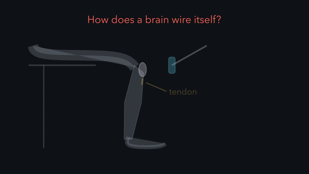 ▶ Watch A Label Is Not a Wire · 4:26
Read the transcript of “A Label Is Not a Wire”
Film transcript: A Label Is Not a Wire
How does a brain wire itself, partner by partner? Start with one small circuit. Tap the tendon below the knee, and the leg kicks. A sensory neuron in the thigh muscle excites the motor neurons of that same muscle. Through an inhibitory interneuron, it also quiets the motor neurons of the opposing muscle. The right partners, with the right signs. Development built every one of those connections. Now scale up. A human brain has about 86 billion neurons. They are joined by something like 100 trillion synapses. The genome that builds them has about 20,000 protein-coding genes. Could the genome simply list the connections? Even using every letter of the genome, the list would be about a million times too long.
So is the trouble giving every neuron its own name? No. Names are cheap. Each extra on-off gene doubles the number of combinations. A few dozen genes could give every neuron its own name. But a name says which cell you are. It does not say whom to connect to.
A label is not a wire. So the genome stores rules. The first is a graded label. Retinal ganglion cells carry a receptor whose amount depends on where they sit in the eye. Their target in the brain carries the matching cue, in an opposing gradient. The second is a local rule. Each growing tip, the growth cone, reads only what is right next to it. Axons with more receptor are kept away from places with more cue.
In our toy model, each axon settles where receptor times cue reaches a set threshold. That rule and the opposing gradients give the right overall order. Real maps also use competition, and more cues. Now take 200 evenly spaced axons and a tenfold gradient. Suppose each reading has an independent random error of about 10 percent. In this toy model, overall order stays high, but neighbouring pairs land in the right order only about 53 percent of the time.
A third rule sharpens that: overproduce, then select. Each axon branches more widely than it needs. Neighbouring cells in the retina tend to fire together. A branch among its retinal neighbours fires in step with them, and together they drive the same target cells. Such branches tend to stay. Branches among strangers tend to retract. The tissue measures this after the connections form, so the genome never has to store it. Here is a test. A goldfish can regrow a cut optic nerve. Block every spike from its eye with tetrodotoxin while the axons grow back. Which part of the map survives: the rough order, or the fine precision?
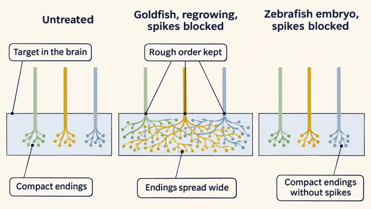
The axons still reached their target, in roughly the right order. But their branches stayed spread over a wide area, instead of clustering tightly. Molecular cues probably placed them. Activity sharpened them. Now block spikes in zebrafish embryos, as their first map forms. The map formed in order, and single arbors stayed small and tight. So the line can fall in different places. But these fish also differ in age, and in regrowing a map versus building one.
The takeaway: the genome stores rules, and the tissue measures the rest. The course follows those rules in three acts: where cells go, how axons find their targets, and who survives.
From the film
- The genome cannot list every connection of a brain, so it stores rules and the tissue measures the rest.
- A label says which cell a neuron is, not whom it should connect to: a label is not a wire.
- Graded labels and local growth-cone rules can give a map its overall order, and activity can sharpen the neighbour order they leave rough.
- Blocking spikes left rough order but spread the endings in regrowing goldfish, while zebrafish embryos formed compact maps without spikes, so where the line falls differs between systems.
Tap the tendon below the kneecap and the leg kicks. For that to happen, sensory neurons in the thigh muscle had to connect to the motor neurons of that same muscle and, through an inhibitory interneuron, to the motor neurons of the opposing muscle. Right partners, right signs. Development made those connections, and on the order of 100 trillion others.
This course asks one question: “How are these neural circuits assembled during embryonic and postnatal development?” This lesson shows why the question is hard, names three developmental strategies, compares two spike-blockade experiments, and lays out the steps the course follows.
One circuit, built right
A neural circuit is a population of neurons joined by synapses to carry out a specific function. The knee-jerk, or stretch reflex, is the simplest one you can feel.
Tapping the tendon stretches the quadriceps, the muscle on the front of the thigh. Sensory neurons sense the stretch. Their endings wrap the specialized muscle fibres inside muscle spindles, and their cell bodies sit in a ganglion beside the spinal cord; they are called Ia afferents. In the cord, each sensory axon excites the motor neurons that drive the quadriceps, and the muscle contracts. The same axon also excites an inhibitory interneuron, which inhibits the motor neurons of the hamstring, the opposing muscle on the back of the thigh. The leg kicks.
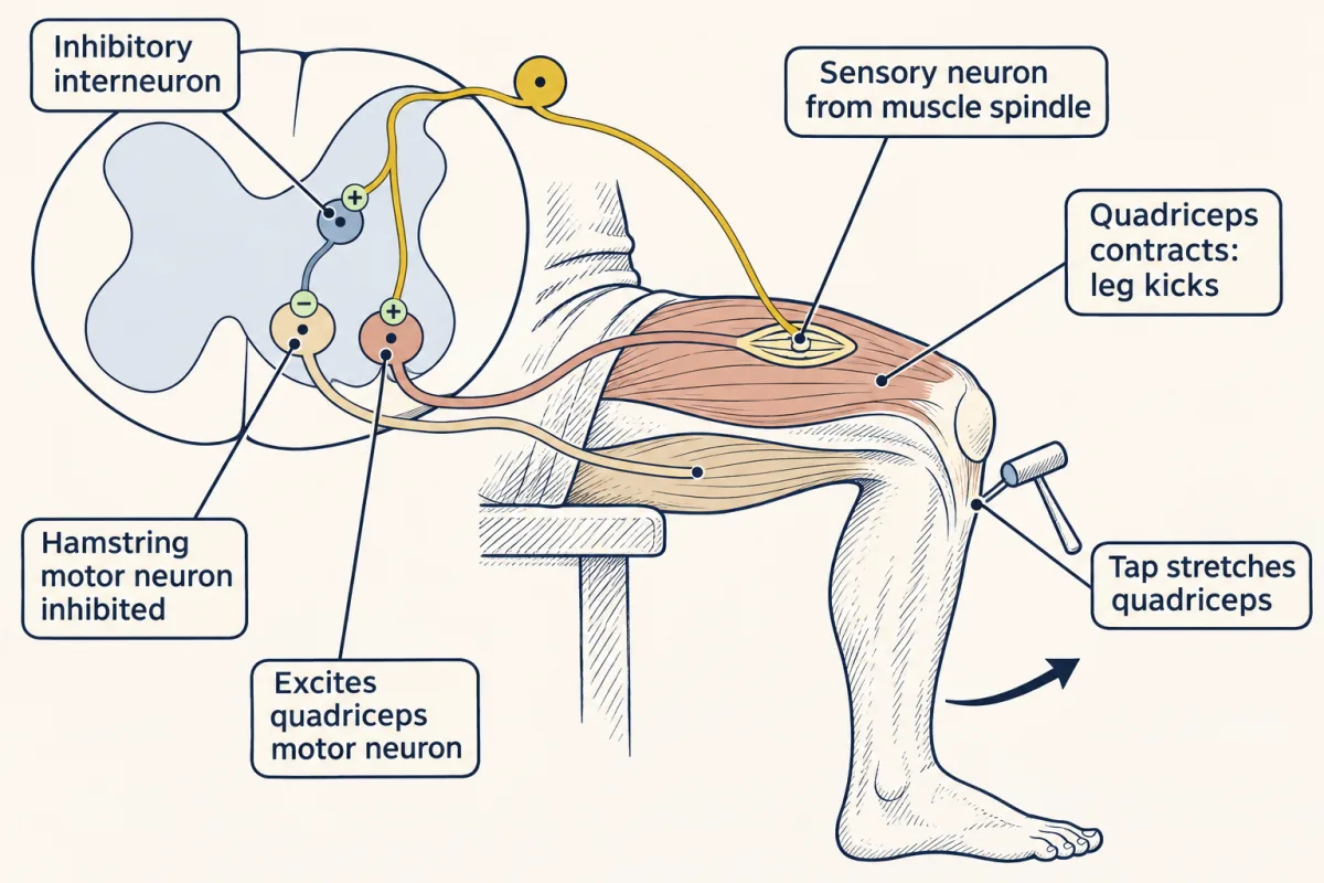
This tiny circuit shows what every circuit in the course has: neurons that work in circuits rather than alone, a direction in which information flows, several kinds of neuron (sensory, motor and interneurons here, each with its own shape), electrical signals, and connections that can be excitatory or inhibitory. One more feature is the developmental one. Connections are selective and precise: each had to be made during development, with the right partner and the right sign.
The wiring problem
Now scale up.
- An adult human brain holds about 86 billion neurons (8.6 × 10¹⁰).
- Each connects to many others, often thousands, so the brain carries on the order of 100 trillion synapses (10¹⁴). Published estimates run from about 10¹⁴ to 10¹⁵, so treat the figure as an order of magnitude.
- The genome that builds them has about 20,000 protein-coding genes, and most of them are also busy running the ordinary business of a cell.
Yet human brains come out wired in much the same way, one after another. Could the genome simply list the connections?
Treat the genome as a file. To name one partner out of 86 billion neurons takes about 36 yes-or-no choices, or bits, because log₂(8.6 × 10¹⁰) ≈ 36.3. A list of 10¹⁴ synapses at 36 bits each needs about 4 × 10¹⁵ bits. The whole genome, all 3.1 billion base pairs and not just the genes, holds at most about 6 × 10⁹ bits: each base is one of four letters, which is two bits. An explicit list is roughly a million times too big (6 × 10⁵ to 6 × 10⁶ times, for 10¹⁴ to 10¹⁵ synapses), before the genome spends anything on running a cell.
wiring list ≈ 10¹⁴ synapses × 36 bits ≈ 4 × 10¹⁵ bits; genome ≤ 3.1 × 10⁹ bases × 2 bits ≈ 6 × 10⁹ bits; shortfall ≈ 10⁶
Predict. A natural first guess is that the hard part is naming: giving each of 86 billion neurons its own tag. Is that the trouble?
Check your prediction
No. Names are cheap. If each gene is either on or off in a cell, each added gene doubles the number of combinations, so 37 genes are enough:
labels = 2ⁿ for n on-off genes; 2³⁷ ≈ 1.4 × 10¹¹, more than the 8.6 × 10¹⁰ neurons
The cost is in the partners. A unique name says which cell a neuron is. It says nothing about which of the other 86 billion cells it should connect to. A label is not a wire.
Real gene families do label neurons, in combinations or gradients, although none is known to give every neuron a unique tag. The clustered protocadherins give a neuron a near-unique identity that lets its own branches recognize and avoid each other. The Eph receptors and their ephrin ligands, membrane proteins that signal where two cells touch, supply graded positional values.
Three strategies instead of a list
So the information that wires a brain has to be compressed into rules that apply in many places at once. It is a little like a city that posts street names in order and a few rules of the road instead of handing every driver a route, except that a driver knows the destination and an axon reads only local cues. Three strategies do most of the work, and each comes with evidence the course returns to.
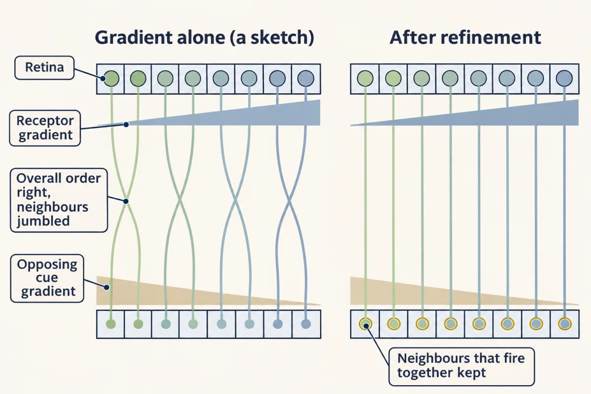
- Graded and combinatorial labels, for position and type. A molecule whose amount rises smoothly across a tissue gives each cell a value for where it sits, with no separate gene for each position. Retinal ganglion cells, the retina’s only output (see The Retina), carry EphA receptors in amounts that depend on their position in the eye. Their target in the midbrain (the superior colliculus in mammals, the optic tectum in fish) carries the matching cue, ephrin-A, in an opposing gradient. Axons with more receptor are kept away from regions with more cue, and a retinotopic map results, in the right overall order: neighbouring cells in the retina connect to neighbouring points in the target (Topographic Maps). What counts is each axon’s receptor level relative to its neighbours’. Two or three gradients at right angles act like map coordinates. Other labels mark kinds of cell rather than positions, so that whole types, not individual cells, find each other.
- Local rules that give global order. A growth cone, the moving tip of a growing axon, senses only its immediate surroundings. It follows a few rules: grow toward more of an attractant, turn away from a repellent, stop at a suitable partner. Followed by many growth cones at once, local rules build a map that spans millimetres (The Growth Cone).
- Overproduce, then select. Make more neurons, branches and synapses than the finished circuit will keep, then remove many of them. What decides which stay is measured after the connections form: which inputs fire together with their neighbours, and which win the limited support, such as nerve growth factor, that targets supply.
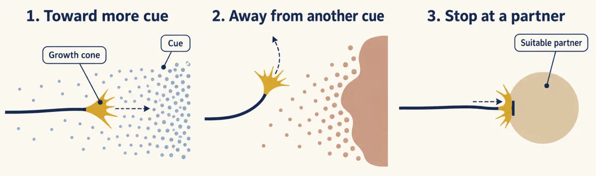
Cues that guide these steps act at different ranges, from direct contact between membranes to molecules that spread through tissue, as the Cell Signaling lesson Signals and How Far They Travel described for signals in general.
The one idea to carry through this course. The genome stores rules, and the tissue measures the rest. In maps like the retina’s projection to the brain, molecular labels, read locally by growth cones, lay out much of the coarse wiring without needing activity. Comparisons made after connections form help set the fine detail and decide which neurons and connections stay.
What the rule covers. It fits large vertebrate maps, the retinotopic map best. Three limits matter.
- Scale. In 1986 John White and colleagues reconstructed the whole nervous system of the worm Caenorhabditis elegans from serial electron micrographs: 302 neurons in the adult hermaphrodite, with about 7,600 synapses and gap junctions. A list of their partners would fit in under a thousandth of the worm’s genome, yet its wiring is still built by guidance cues and partner recognition rather than read from a list. So rules are not used only for lack of space.
- Matching labels. Some precise connections, down to particular partners and layers, form without activity, by matching labels between partner types.
- Where the line falls. It differs between systems, as the experiments below show.
Why one noisy gradient gives only rough order
If gradients already give a map, why is the third strategy needed? One reason is that reading a gradient is noisy.
Take a deliberately simple model, a sketch that asks only how much order one gradient can carry, not how real growth cones read it. A receptor gradient across the retina and a cue gradient across the target each change tenfold from one edge to the other. Each growth cone settles where its reading of receptor times cue reaches a set level, and each reading is off by about 10 percent at random.
Predict. Two hundred axons start in order across the retina. Do they land in the right overall order across the target? Do neighbouring axons land in the right order?
Check your prediction
The overall order comes out nearly perfect: in simulations of the sketch, the rank correlation between start and landing position (1 means perfect order) was about 0.99. Neighbours do barely better than chance. On average about 106 of the 199 neighbouring pairs land in the right order, and single runs mostly give 99 to 113, where chance alone gives about 100.
The reason is resolution. With fractional error σ in each reading and an F-fold gradient:
resolvable positions ≈ ln F ÷ 2σ; F = 10, σ = 0.1 → about 12; F = 100, σ = 0.05 → about 46
A mouse retina has about 45,000 to 70,000 ganglion cells. Laid out as a square grid, that is about 210 to 260 along each side, so the sketch’s 12 to 46 positions are about 5 to 23 times coarser. That is only a yardstick: types, density and arbors overlap, so a real map does not need one position per cell.
So in the sketch, local order stays nearly random. Neighbouring retinal cells tend to fire together; before vision begins, much of that correlated firing comes in spontaneous waves that sweep across the retina (Activity Before Experience). A branch that lands among the endings of its retinal neighbours fires in step with them, so together they drive the same target cells, and that branch tends to be kept. A branch that lands among strangers fires out of step and tends to be lost. Together with competition, this can sharpen the neighbour order that a gradient leaves rough.
Testing the split: block the spikes
The guiding idea makes a prediction for maps built this way. Remove activity while a map forms, and the coarse order should survive, while any precision that depends on activity fails. The tool is activity blockade. Tetrodotoxin blocks voltage-gated sodium channels, so neurons cannot fire action potentials, or spikes. A connection that still forms without spikes did not need them; one that forms but fails to become precise needs activity.
In an adult goldfish, a cut optic nerve regrows, so retinal axons grow back to their target in the brain and rebuild the map. Inject the eye repeatedly with tetrodotoxin while they do.
Predict. With every spike from the eye blocked, which survives: the rough order of the map, the fine precision of each axon’s ending, or both?
Check your prediction
Only the rough order. The axons still reached the target in roughly the right order, but each axon’s terminal branches stayed spread over a wide area, while in untreated fish they cluster tightly. So rough targeting can be built without action potentials, probably guided by molecular cues, and sharpening the map needs activity.
Predict. Now block spikes in developing zebrafish embryos, while the retinal map forms for the first time. Expect the same result?
Check your prediction
No, not in the early window measured. In zebrafish embryos with spikes blocked from about the time retinal axons began to grow, the map formed in order, single axons made arbors as small as in untreated embryos, and neighbouring axons ended in equally compact clusters (Stuermer and colleagues, 1990). So in that first embryonic map, fine precision formed without spikes too. The two experiments also differ in species, in stage, and in regrowing a map against building one for the first time, so these results alone do not say which difference matters. They set different limits on what needs spikes in the two conditions tested; in both, guidance and refinement use genetically encoded rules acting on local information.
Overproduce, then select, across a human life
A conventional electronic circuit is assembled before it is switched on, and once it is finished its wiring does not change with use. A developing neural circuit works while it is being built. Embryonic neurons fire, and connections made early carry signals while later ones are still growing. Those signals, and later experience, help decide which connections stay.
If the human cortex overproduces and then selects, synapses should rise and then fall. In 1979 Peter Huttenlocher counted synapses per unit volume, their density, by electron microscopy in a region of human frontal cortex, in tissue from people of many ages.
Predict. What does synapse density do between birth and adulthood?
Check your prediction
It rises, then falls. Synapse density was already high at birth, rose during infancy, peaked at about one to two years of age at roughly half again the adult value, and then declined through childhood and adolescence. The cortex appears to make more synapses than it keeps. Density counts alone cannot show what decides which synapses stay, and a density is not a total count (see Going deeper).
The timing differs between regions. The course returns to this, and to what happens “when assembly goes wrong”, in later lessons.
The roadmap: from induction to refinement
“Neural circuits develop in several steps.” The course follows them in order. The last column is a rough guide to what is most on show at each step, usually one of the three strategies.
| Step | What happens | Course unit | Strategy most on show |
|---|---|---|---|
| 1. Induction | Part of the ectoderm, the embryo’s outer layer of cells, is told to become neural tissue. | 2: Becoming neural | Signals that specify neural fate |
| 2. Patterning | That tissue is divided into regions along its long axis and from back to belly. | 3: Coordinates | Graded labels for position |
| 3. Generation of neurons and glia | Dividing precursors make neurons and their support cells, the glia, in a set order. | 4: Making neurons | Labels for type |
| 4. Migration | Young neurons move from where they were born to where they will work. | 5: Cells on the move | Local rules |
| 5. Axon growth and guidance | Most neurons send out an axon, which steers toward its target. | 6: Axons find their way | Local rules reading labels |
| 6. Target selection | The axon picks a region, then particular cells within it. | 6: Axons find their way | Labels and local rules, down to particular partners |
| 7. Naturally occurring death | Many of the neurons made die, shaped by competition for support from their targets. | 7: Survival and competition | Overproduce, then select |
| 8. Synapse formation | Contacts become working synapses. | 8: Building synapses | Matching labels and local rules |
| 9. Activity-dependent refinement | Use sharpens the connections and removes some. | 9: Experience refines the wiring | Overproduce, then select |
The steps overlap in time, and many of them reuse the same signals: Wnt, bone morphogenetic protein (BMP), Hedgehog and Notch, the pathways of the Cell Signaling course.
The course gathers them into three acts. Act 1 is coalescence: where cells go, and how scattered migrating cells gather into ganglia and layers. Act 2 is guidance: how axons find their targets. Act 3 is competition: who survives. That act opens with the question “Why make neurons just to kill them?”, and with nerve growth factor, a protein made by targets that neurons compete for, which the Cell Signaling lesson Finding a Signal traced to its discovery.
Design problem
You have about 20,000 genes and must wire a visual system in which each retinal axon ends at the right point in the brain, preserving the layout of the retina. Propose two strategies that need far fewer than one gene per connection. Then design one experiment that tells whether forming a given connection needs neural activity, and one that asks whether it needs visual experience in particular.
Saved in this browser only.
One way to do it
Strategy 1: opposing gradients. As in the gradient sketch above, give the retina a receptor gradient R(x) = R₀Fˣ and the target an opposing cue gradient L(y) = L₀F⁻ʸ. Let each axon settle where R × L reaches the same threshold; with the threshold set at R₀L₀, an axon from position x lands at y = x. That one rule orders many axons with one receptor gene and one cue gene, although with the sketch’s noise and spacing neighbours land in poor order. Real maps also use competition, relative receptor levels and additional cues.
Strategy 2: overproduce, then select. Let each axon branch over a wider area than it needs. Branches whose synapses drive target cells together with correlated inputs from retinal neighbours are more likely to stabilize; less effective branches are more likely to retract. Together with molecular cues and competition, this can sharpen the map without any gene for each connection.
Experiments. Block activity in the eye during development, for example with repeated injections of tetrodotoxin. To remove visual experience while spontaneous activity continues, raise the animal in the dark instead. A connection that forms normally without what was removed did not need it, and molecular cues are the likely guide; one that lands in the right rough place but fails to sharpen needs it to refine. As the goldfish and zebrafish results show, the answer depends on the system.
Going deeper
Where the numbers come from
The neuron count comes from a 2009 study by Frederico Azevedo, Suzana Herculano-Houzel and colleagues, who counted cell nuclei in the brains of four adult men and found 86.1 billion neurons, give or take about 8 billion. It is an estimate from a small sample, and the most widely cited direct count. In 2003 Bente Pakkenberg and colleagues estimated about 1.5 × 10¹⁴ synapses in the human neocortex alone. The clustered protocadherins are three neighbouring gene clusters holding more than 50 genes in the human genome, and the Eph receptors and their ephrin ligands number around twenty between the two sides.
Why count bits rather than genes
The wiring problem is often stated as a ratio: the genes are fewer than the neurons by a factor of millions and fewer than the synapses by a factor of billions, so a list with one instruction per synapse would be billions of times longer than the list of genes. That comparison mixes units. One gene can act at many synapses, so a gene count does not measure how much a genome can say. The comparison in bits, which counts every base of the genome, avoids the objection.
The gradient sketch in full
In the sketch, a ganglion cell at position x across the retina carries receptor R, which changes F-fold from one edge to the other; the target carries cue L, which changes F-fold the other way. The axon settles where the product R × L reaches a threshold, and its reading has a random Gaussian fractional error with standard deviation σ. An error of σ in the reading moves the landing point by about σ ÷ ln F of the target’s width, and two positions can be told apart when they sit about two such errors apart (such a pair lands in the right order about 92 percent of the time), which gives about ln F ÷ 2σ positions. The simulations used 200 evenly spaced axons with F = 10 and σ = 0.1. The sketch assumes threshold reading, a single exponential gradient and independent errors, so it shows why refinement could be needed rather than how noisy real growth cones are.
Axons read relative, not absolute, levels
The sketch’s threshold rule is not how the retinal map works. In the Isl2–EphA3 knock-in, extra EphA3 was added to about half the ganglion cells, and the map duplicated: wild-type axons shifted too, although their own receptor levels were unchanged. Mapping follows the receptor level of an axon relative to the axons it competes with (Brown et al., Cell, 2000; Reber, Burrola and Lemke, Nature, 2004). In developing rats, retinal axons also overshoot their final position and form side branches, preferentially in a broad region that includes the correct one; remodelling then removes the misplaced branches and builds up the arbor at the correct site (Simon and O’Leary, 1992). Topographic Maps follows these experiments.
Precise wiring without activity
In the retina’s inner plexiform layer, the thin band where bipolar, amacrine and ganglion cells connect, partner types meet in the same sublayer, guided in part by matching adhesion proteins such as the Sidekicks (Choosing a Partner). In the spinal cord, which motor neurons a stretch-sensing sensory neuron contacts is set largely by the motor neurons’ position. Much of the early wiring of flies and worms also forms without activity.
The worm’s list
White and colleagues counted roughly 5,000 chemical synapses between neurons, 2,000 onto muscle and 600 gap junctions in C. elegans, about 7,600 contacts. A partner list needs 9 bits for each end (enough to name any of the 302 neurons or 95 body-wall muscles) and 2 bits for the kind of contact: 7,600 × 20 ≈ 1.5 × 10⁵ bits, against a genome of about 2 × 10⁸ bits, under a thousandth. It leaves out where on each cell a contact sits and how strong it is. Its wiring is highly stereotyped, but the connectomes of individual worms differ in a sizeable minority of connections, mostly weak ones. An open question is how much of any mature circuit is specified before activity begins.
Goldfish and zebrafish
The zebrafish result covers the first embryonic map. Whether later refinement of fish arbors needs activity has been revisited since, so it does not show that all refinement in zebrafish is activity-independent.
Density is not a total count
The cortex grows during childhood, so a falling density could partly reflect tissue growth: it is consistent with synapse loss but does not by itself prove it. Studies in animals that follow the same dendritic spines over time show the loss directly.
Synapse density in different cortical regions
In a 1997 study the peak came at about 3 months in auditory cortex and after 15 months in prefrontal cortex, and a 2011 study found spine loss in prefrontal cortex continuing into the third decade of life.
How many kinds of retinal ganglion cell?
How many kinds of neurons must be wired? Take retinal ganglion cells. Early anatomists sorted them into a few classes by shape. A 2002 survey of 520 mouse retinal ganglion cells sorted them by shape into four main groups, and a 2019 single-cell survey of gene expression in mouse reported 46 types, so the count depends on the method. Types differ in the combination of brain targets they reach, and most targets receive several types.
Your notes
Select any text in the lesson to highlight it or add a note to it. Your highlights and notes are saved in this browser and collected in your notebook.
This browser is not letting the site save anything (a private window or strict privacy settings), so highlights and notes will be lost when you leave the page.
How we measure it
Isotropic fractionator
Brain tissue is dissolved in detergent into an even suspension of free nuclei. Counting the nuclei in a sample gives the total number of cells, and staining with an antibody to the neuronal nuclear protein NeuN gives the fraction that are neurons.
Serial-section electron microscopy
Tissue is cut into a long series of very thin sections, each imaged in the electron microscope, and each neuron is traced from section to section. It resolves single synapses, so it can map connections or count synapses in a known volume.
Activity blockade
A drug such as tetrodotoxin, which blocks voltage-gated sodium channels, is applied so that neurons cannot fire action potentials. A connection that still forms is built without action potentials; one that forms but fails to become precise needs activity.
Practice questions on this lesson (3) → MCAT-style, original, each with an explanation
Where this lesson fits
After thisStudy next
- The Growth Cone: The Tip That Steers the AxonThis course · Lesson 3
It shows how a growth cone reads only local cues, the second strategy this lesson names.
- Topographic Maps: Sperry's Eye and Eph GradientsThis course · Lesson 26
It follows the Eph and ephrin gradient experiments that this lesson uses to show graded labels giving a map.
- Activity Before Experience: Spontaneous Retinal WavesThis course · Lesson 38
It takes up retinal waves, which sharpen the neighbour order that one noisy gradient leaves rough.
Elsewhere on the siteFilms, simulations and method films in other courses
- Where Every Command EndsFilm · Neuroscience
It shows the stretch reflex circuit and why the connection from sensory axon to motor neuron matters.
- Centre and surroundSimulation · Neuroscience
It shows how retinal cells are organized, the system whose map this lesson tests with blocked spikes.
Suggested by an AI model from the lessons themselves, then checked. How we use AI
Finish line
Test yourself
8 questions
Practice and MCAT-style, with explained answers.
Next · Lesson 2
Seeing Neurons: Golgi, Cajal and the Neuron Doctrine
Are neurons separate cells that touch, or one fused network? The neuron doctrine says separate, and it took a new stain, a lot of embryos and the electron microscope to show it. Two men looked at the same stained brain and saw two different organs. Who was right, and how could anyone tell?
Continue →