Sensory Systems · Unit 6: Hearing and balance
The Cochlear Amplifier and Otoacoustic Emissions
Rewritten on : new text, flashcards and film. Your notes and highlights stay, but the text around them may have moved.
A microphone sealed in a healthy ear canal can record sound that your own cochlea made. What does that sound tell us about the amplifier, and what can it not tell us?
Pause when the reading reaches a film, and offer to play it. Saved on this device.
Watch the film now, or keep listening
Builds on:Five Ways to Turn a Stimulus into a CurrentThe Hair Cell's Transduction ChannelWhy these?
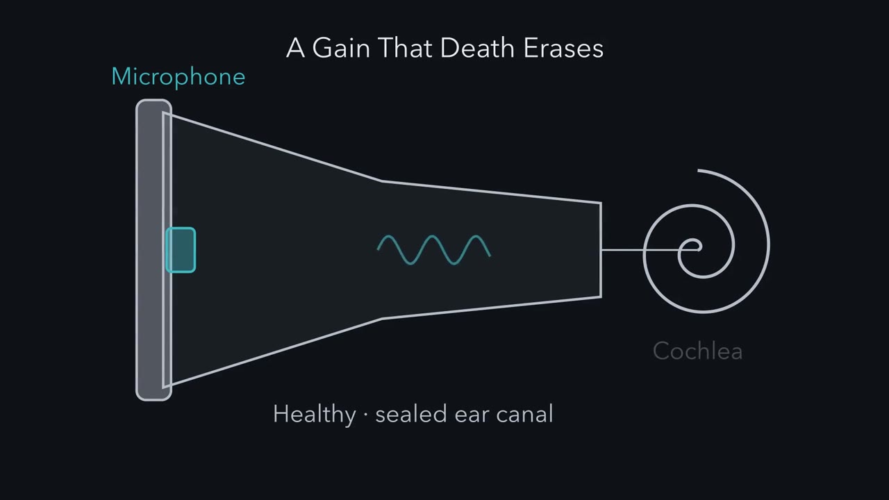 ▶ Watch A Gain That Death Erases · 2:42
Read the transcript of “A Gain That Death Erases”
Film transcript: A Gain That Death Erases
A microphone in a healthy ear canal can record sound the cochlea itself made. Where does it come from? Start with a cochlea that has no help. Sound sets up a travelling wave along the basilar membrane. In a living ear, at soft levels, each place moves most for one frequency, its characteristic frequency. The wave peaks there and dies out just beyond. After death the wave remains, but weak and broadly tuned, and its peak can shift. Now pick one place. Play a tone at its characteristic frequency, and raise the level in steps. After death, 10 dB more sound gives 10 dB more motion. That straight line is linear. Predict. Where does the living ear differ most from the dead one, at soft levels or loud ones?
At soft levels. A soft tone moves the living membrane tens of decibels more. As the tone gets louder, the living response grows slowly, often 2 to 5 dB for every 10. At the loudest levels, the two curves come close together.
The gap between the curves is the cochlear amplifier. In mammals, it depends on outer hair cells. The gain is large only near the characteristic frequency, so it sharpens the peak as well as raising it. Here is the one idea. Outer hair cells add energy to the wave near its peak. The gain they give is large for soft sounds, small for loud ones, and gone after death. Sensitivity, sharp tuning, compressive growth and the returning sound are four signatures of that one gain. At the very softest levels, the gain stops rising. It levels off at its maximum. Why want a gain that shrinks? Suppose the response grows 2.5 dB for every 10. If that slope held over 60 dB, a quiet room to a shout would fit into 15 dB of motion.
That is a thousandfold range of sound pressure, fitted into less than a sixfold range of motion. Outer hair cells push with a motor protein in their side wall, called prestin. How does a cell push that fast? Take this with you. The living cochlea adds a gain that is large for soft sounds, and death erases it.
From the film
- The cochlear amplifier is the gain of the living cochlea over the dead one, and in mammals it depends on outer hair cells.
- That gain is large for soft sounds, small for loud ones and gone after death.
- Sensitivity, sharp tuning, compressive growth of motion and the returning sound are four signatures of that one gain.
A microphone sealed in a healthy ear canal can record sound that the cochlea itself made. What does that sound tell us about the amplifier, and what can it not tell us?
That faint sound is how newborns are screened for hearing loss. Start with what a cochlea does without any help. Sound entering the inner ear sets up a travelling wave along the basilar membrane. Measured with soft sounds in a healthy ear, each place along the cochlea moves most for one frequency, its characteristic frequency: high frequencies near the base, low ones near the apex. The wave grows as it travels, peaks at the place that matches its frequency, and dies out just beyond. A cochlea that is mechanically intact but no longer alive still carries the wave, but weakly and with broad tuning, and its peak can shift. Call that the passive cochlea.
The core lesson hearing and balance showed that outer hair cells (the three rows that amplify; the single row of inner hair cells sends most of the signal to the brain) shorten and lengthen with voltage, that the protein prestin in their side wall is the motor, and that a knock-in mouse supports a requirement for its motility. This lesson starts there: what the living cochlea adds to the passive one, the engine that adds it, the motor’s electrical fingerprint and structure, the sound a healthy ear sends back out, the frog hair bundle as a possible second engine, and where along the cochlea the gain is gathered.
A gain that death erases
Compare a living cochlea with the same cochlea after death. Measure the basilar membrane at one basal place, play a tone at that place’s characteristic frequency, and raise the sound level in steps. Plot both on decibel scales: sound level along the bottom, motion up the side.
After death, the motion grows in proportion to the sound. Ten dB more sound gives 10 dB more motion, so the plot is a straight line with a slope of 1. A system like that is linear: its output keeps a fixed proportion to its input. A system whose output does not keep that proportion is nonlinear.
Predict. In the living ear, would you expect the biggest difference from the dead ear at soft levels or at loud ones?
Check your prediction
At soft levels. In sensitive recordings from the base of the cochlea (reviewed by Robles and Ruggero, 2001), a soft tone at the characteristic frequency moves the living membrane tens of decibels more than the same membrane after death; louder tones close the difference, as the table below sets out. Well below the characteristic frequency, the living and dead curves are nearly the same.
Read the two curves side by side. The table is a schematic of their shapes, not data.
| Sound level, at the characteristic frequency | After death | Living | Living minus dead (the gain) |
|---|---|---|---|
| Softest | grows 10 dB per 10 dB | grows about 10 dB per 10 dB, like the dead curve, but sits tens of dB higher | largest, and steady: the plateau |
| Soft to moderate | grows 10 dB per 10 dB | grows slowly, often 2 to 5 dB per 10 dB | shrinks as the sound gets louder |
| Loudest | grows 10 dB per 10 dB | comes close to the dead curve | small |
On decibel axes the gain is the vertical gap between the curves, and where the living slope is below 1 and the dead slope is 1, the gap closes as the level rises. That gap is the cochlear amplifier, the active process that lets the ear detect weak sounds, separate nearby frequencies and handle a wide range of loudness. In mammals it depends on outer hair cells. Because the gain is large only near the characteristic frequency, it sharpens the peak of the travelling wave as well as raising it.
The one idea to carry through this lesson. Outer hair cells add energy to the travelling wave near its peak. The gain they give, the living response compared with the dead one, is large for soft sounds, small for loud ones and gone after death. The ear’s sensitivity, its sharp tuning, the compressive growth of its motion and the sound it sends back out are four signatures of that one vulnerable gain.
The idea holds at and near the characteristic place in a living mammalian cochlea, and the curves above come from basal sites. The gain is a ratio, so a falling gain does not by itself mean the cells do less work at high levels. The gain has a plateau: at the very softest levels it stops rising and levels off at its maximum, and the response is linear again. It does not say how the work is split between the cell body and the hair bundle, how far along the cochlea the gain is gathered, or whether the motor pushes on every cycle at the highest frequencies.
Why would an ear want a gain that shrinks? Suppose the living response grows 2.5 dB for every 10 dB of sound across the middle of the range, a slope of 0.25 (an illustrative value). If that slope held over 60 dB of sound, from a quiet room to a shout, the motion would span only 60 x 0.25 = 15 dB: a thousandfold range of sound pressure fitted into under a sixfold range of motion. At a slope of 0.5 the same range would take 30 dB. A narrow range of motion is thought to help the hair cells and nerve handle a wide range of loudness.
The engine: from a bent bundle to a pushing cell
Read the transcript of “From a Bent Bundle to a Pushing Cell”
Film transcript: From a Bent Bundle to a Pushing Cell
How does one cell push on a sound wave, many thousands of times a second? The chain has five links. Sound bends the hair bundle back and forth. Bending toward the tallest stereocilia opens more transduction channels. Current flows in, so the voltage rises and falls with the bundle. The voltage moves charge inside prestin, which changes shape. The cell shortens and lengthens in step, and pushes on the organ of Corti. Why voltage? A 20 kHz tone completes a cycle every 50 microseconds. An amplifier working on every cycle cannot wait on a slow chemical step, such as ATP hydrolysis. Voltage has limits too. The membrane smooths fast voltage changes.
In simple estimates, its cutoff lies far below the highest frequencies basal cells amplify. How much that limits the amplifier is still argued. How can you watch prestin's charge move? Measure capacitance, the charge moved per change in voltage. In the simplest model, each prestin flips between two states, and voltage tilts the odds. So its charge moves along an S-shaped curve, mostly near its midpoint. The slope of an S peaks at its middle. So the extra capacitance is a bell, called nonlinear capacitance. Its steepness is set by z, the effective charge that moves per prestin. Predict. If z doubles, does the bell get wider or narrower?
Narrower. A larger z makes the S steeper. The width of the bell scales as one over z. Take the gerbil fit. At 50 mV above the midpoint, about 80% % of prestin is in the contracted state. The bell there is 64% % of its peak. This reads charge movement, not the force or power a hair cell produces. Structures of purified prestin suggest an area motor. But each is a candidate end state, not a working motor. Is the motor needed? In a prestin knock-in mouse, transduction and cell mechanics were normal. Yet amplification was lost. So the cell body's motility is necessary. In an excised frog organ, a hair bundle can also add energy. How the work is split between bundle and cell body in mammals has not been established.
Take this with you. Bundle, channel, voltage, prestin, push. The bell is the motor's electrical fingerprint.
From the film
- The outer hair cell turns sound into force through a chain: bundle bending, transduction current, voltage, prestin shape change, and a push on the organ of Corti.
- Nonlinear capacitance is the electrical fingerprint of prestin's charge movement, and it does not measure the force or power a hair cell produces.
- In a prestin knock-in mouse amplification was lost while transduction and cell mechanics were normal, so cell-body motility is necessary; how the work is split with the bundle in mammals is not established.
To add energy near the peak, an outer hair cell must turn sound into force, fast. Outer hair cells are thought to add energy on each cycle of a sound. The chain has five links:
- Sound bends the hair bundle back and forth.
- Bending toward the tallest stereocilia opens more mechanically gated transduction channels, and bending the other way closes some of those open at rest (the hair-cell transduction channel).
- Transduction current flows into the cell, so the voltage rises as channels open and falls as they close.
- The voltage moves charge inside prestin, and prestin changes shape.
- The cell shortens as it depolarizes and lengthens as it hyperpolarizes, and pushes on the organ of Corti, the strip of cells on the basilar membrane that holds the hair cells.
Speed rules out some designs. A tone at 20 kHz, near the top of the human range, completes a cycle every 50 microseconds. An amplifier that adds energy on every cycle cannot wait for a slow chemical step such as ATP hydrolysis each time, so the outer hair cell uses a protein that responds to voltage directly.
Voltage has a speed limit of its own. The membrane’s resistance and capacitance smooth fast voltage changes, so less of the voltage swing reaches prestin as frequency rises. In simple electrical estimates, this filter’s cut-off lies far below the high frequencies that basal outer hair cells help amplify, though its value depends on the cell’s place along the cochlea and on conditions. Prestin’s own kinetics are finite too. How much cycle-by-cycle force reaches high frequencies, and so how much this limits the amplifier in the living cochlea, is still argued (reviewed by Altoè and Shera, 2023).
Prestin belongs to the SLC26 family of anion transporters (membrane transport), yet in the outer hair cell it works as a motor.
Reading the motor’s fingerprint: nonlinear capacitance
How do you see charge move inside a protein in a living membrane? Through capacitance, the charge moved per unit change of voltage, C = dQ/dV. An ordinary membrane stores charge in proportion to voltage, so its capacitance is constant. Prestin adds charge of its own. In the simplest model, each prestin flips between two states and voltage tilts the odds between them, so the charge moved within the protein follows an S-shaped curve against voltage: little moves far from the midpoint, and most moves near it. The slope of that S is largest at its midpoint and falls on both sides, so the extra capacitance is a bell.
That bell is nonlinear capacitance (NLC), measured in whole-cell voltage clamp, where a pipette holds the cell at chosen voltages. The usual reading is that it reports voltage-dependent displacement of charge in the protein. Depolarization shifts prestin toward a contracted state, the state associated with outer hair cell shortening.
The two-state model uses the occupancy f of the contracted state, a half-activation voltage Vh, and an effective valence z, the charge that moves per prestin, counted as if it crossed the whole membrane:
f(V) = 1 / (1 + exp(-z (V - Vh) / (kT/e))), normalized NLC = 4 f (1 - f)
Here kT/e is the thermal voltage, which sets the voltage scale, and 4f(1 - f) is the slope of f, scaled so that the peak is 1.
Predict. If z doubles, does the bell get wider or narrower?
Check your prediction
Narrower. A larger z makes the S steeper, so the charge moves over a smaller range of voltage. The width of the bell at half its height scales as 1/z: in this model it is about 128 mV at z = 0.70 and about 64 mV at z = 1.40.
Worked problem. Butan and colleagues fitted gerbil prestin in an induced HEK cell line with Vh = -112 mV and z = 0.70 (an effective charge, not a count of transported chloride ions). Assume 295 K, a two-state equilibrium, no linear capacitance and no kinetics, so kT/e = 25.42 mV. What are the occupancy and normalized NLC at Vh and at -62 mV?
Step 1: at Vh. The exponent is zero, so f = 0.5 and normalized NLC = 4 x 0.5 x 0.5 = 1, the peak.
Step 2: at -62 mV. The shift is -62 - (-112) = +50 mV. The exponent is -0.70 x 50 / 25.42 = -1.377, so f = 1 / (1 + 0.2523) = 0.798. Occupancy rose by 0.298.
Step 3: capacitance. Normalized NLC = 4 x 0.798 x 0.202 = 0.644, about 64 percent of the peak.
Step 4: check. At -162 mV, 50 mV hyperpolarized from Vh, f = 0.202 and NLC is again 0.644.
So the bell maps where prestin’s charge, and so its shape, is most sensitive to voltage. These numbers describe a cell line at room temperature under the stated assumptions, and Vh there is not the operating voltage of an outer hair cell in the cochlea; it shifts with conditions. Nor do they say how much force or power a hair cell produces.
Hollow orange circles mark the mirror voltage, the same distance on the other side of Vh.
- V − Vh
- +50 mV
- Exponent −z(V − Vh)/(kT/e)
- −1.377
- Occupancy f (contracted)
- 0.798
- Change in f from Vh (0.5)
- +0.298
- NLC as a fraction of peak
- 0.644
In this sketch: two-state equilibrium, no linear capacitance, no kinetics, kT/e = 25.42 mV (295 K). Vh = −112 mV and z = 0.70 are the values fitted to gerbil prestin in an induced HEK cell line at room temperature (Butan and colleagues, 2022). The curves are computed from the lesson’s equation, not recorded.
Keep this rule: the bell reports how the protein’s charge responds to voltage in a cell line. It does not say how much force or power a hair cell produces.
What the structures can and cannot show
Three structural papers appeared within about a year, in 2021 and 2022, on human, dolphin and gerbil prestin, each with a different emphasis. They agree that the protein changes shape and that the change is coupled to the membrane. The human and gerbil structures show a dimer whose two halves swap domains. In human prestin, the structure solved in chloride and the one solved in salicylate, a drug that inhibits prestin, differ by about 200 square angstroms (2 square nanometres) in the mean cross-sectional area the dimer occupies in the membrane. That suggests an area motor: a protein that changes how much membrane it takes up. The proposal is that when many prestin molecules in the side wall change their area together, the wall’s area changes, and the cell’s length with it.
The groups differ on what senses voltage. The dolphin study proposed a composite sensor: a bound anion, the charged residues that hold it, and a helix dipole. The gerbil study found that a mutant at the anion site, S398E, kept its nonlinear capacitance in 20 millimolar salicylate, which the authors argued is hard to reconcile with chloride alone as the voltage sensor.
Read these as complementary views, not one settled movie. Every structure is of purified protein under chosen anion or drug conditions, and the gerbil map did not resolve a bound chloride. Butan and colleagues cautioned that salicylate- or sulfate-stabilized structures could differ from the shapes of a voltage-driven protein. Each structure is a candidate end state, not a recording of a working motor. The 200 square angstrom figure compares two such states. It is not a stroke measured in a hair cell, and it is not mechanical work.
The sound that comes back
Read the transcript of “The Sound That Comes Back”
Film transcript: The Sound That Comes Back
Why would a healthy ear send sound back out? And what can a screening test learn from it? In 1978, Kemp played brief clicks into human ear canals and averaged the response. A slowly decaying sound remained after each click. In the ears tested with cochlear deafness, it was absent. Some emissions come from reflections of the travelling wave. Others come from the cochlea's nonlinearity. Picture a curve that acts on the sound wave instant by instant. It passes small inputs and flattens large ones. Feed it two tones, at 2,000 and 2,400 hertz. Predict. What comes out, besides the two tones you put in?
New tones. Where the two tones add up to a big peak, the curve squashes it. A cubic term mixes two of the first tone with one of the second. That makes 1,600 hertz, among other new tones. In ear-canal tests, that one is usually the largest.
Predict again. Play the same tones at a moderate level into a cochlea after death. What comes back? Usually little or nothing, at these levels. The living drive and amplification are gone. That does not mean every nonlinearity in the transduction channel has vanished. That is the one idea at work. The same vulnerable process gives the gain and makes the emission. A fast, saturating curve makes new tones whenever the input reaches its curved part. What ties this one to outer hair cells is that, at screening levels, it fails when they fail. A fast, saturating curve makes new tones when they fail. Newborn screening uses emissions. A pass shows outer hair cells can make an emission through the middle ear.
It does not show intact hearing. In auditory neuropathy, the brainstem response can be absent or very abnormal. One question stays open. How far along the cochlea is the gain gathered? A second tone can lower the response to first one. Changing its frequency changes where it acts, which helps map the gain. Take this with you. A living cochlea's nonlinearity makes new tones, and a microphone in the ear canal can hear them.
From the film
- A fast nonlinearity in a living ear makes new tones, such as 2f1 minus f2, that a microphone in the ear canal can record.
- At screening levels the distortion product fails when outer hair cells fail, which is what ties it to the amplifier.
- A passed emission screen shows outer hair cells can make an emission, not that hearing is intact, because auditory neuropathy can present with a normal emission.
Now return to the microphone in the ear canal. Kemp (J. Acoust. Soc. Am., 1978) studied human ears in vivo. Brief acoustic impulses were delivered to the closed ear canal and the canal response was signal-averaged. Beyond 5 milliseconds after the stimulus, a slowly decaying component remained, with a decay constant over 12 ms. In the ears with cochlear deafness that were tested, it was absent. That supports a cochlear source. It does not identify a motor.
Emissions come in two main kinds (Shera and Guinan, 1999). Click-evoked emissions like Kemp’s arise mainly from reflection of the travelling wave off small irregularities near its peak. Distortion-product emissions arise mainly from the cochlea’s nonlinearity. Both depend on the active process.
A distortion-product emission uses two tones, f1 and f2, played together. To see why it should exist, picture a curve that acts on the waveform instant by instant: it passes small inputs faithfully and flattens large ones. In the living cochlea the main such curve is thought to be the transduction channel itself, whose current saturates for large deflections of the bundle. Feed the curve the sum of two tones.
Predict. What comes out besides f1 and f2?
Check your prediction
New frequencies. Where the two tones add up to a large peak, the curve squashes it, and the squashed waveform contains frequencies the stimulus did not. A linear system gives back only f1 and f2. A curve with a cubic term, such as y = ax - bx³, mixes two copies of f1 with one of f2 and makes 2f1 - f2, among other products. In the ear canal, with the stimulus settings used in testing, 2f1 - f2 is usually the largest of them. Suppose f1 = 2,000 Hz and f2 = 2,400 Hz in an invented example: 2 x 2,000 - 2,400 = 1,600 Hz, a frequency the stimulus did not contain.
Predict. Now play the same two tones at a moderate level into a cochlea after death. What comes back at 1,600 Hz?
Check your prediction
Usually little or nothing: at these moderate levels the distortion product in the ear canal is greatly reduced or undetectable after death. The living electrical drive and the mechanical amplification are gone. That does not mean every nonlinearity has vanished: in mice lacking prestin, distortion-product emissions still appear at high levels (Liberman, Zuo and Guinan, 2004), consistent with a nonlinearity that does not need the motor. This is the one idea at work: the same vulnerable process that gives the gain also makes the emission. The logic runs one way, though. An instantaneous saturating curve makes new frequencies whenever the two tones together reach its curved part, so the mathematics alone does not point to outer hair cells. And a slow volume control could compress motion without making new tones, so a compressive input-output curve by itself does not prove the waveform is distorted. What ties the distortion product to outer hair cells is that, at the low-to-moderate levels used for screening, it is vulnerable: it fails when they fail.
A screening pass shows that outer hair cell activity can produce an emission through the middle ear. It does not show intact hearing, because auditory neuropathy can present with a normal emission and an absent or very abnormal auditory brainstem response, a scalp recording of synchronous firing in the auditory nerve and brainstem (NIDCD). Emission and brainstem tests probe different stages.
The brain can also turn the gain down, through efferent fibres that end on outer hair cells.
A second engine? The frog hair bundle
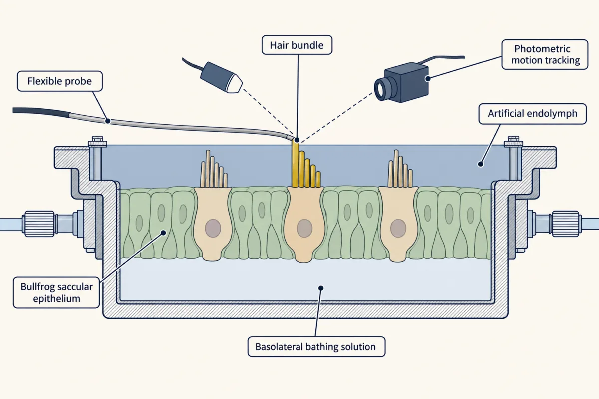
Outer hair cell bodies are not the only candidate. Martin and Hudspeth (PNAS, 1999) used adult bullfrog saccular epithelium in vitro, with the otolithic membrane removed. A two-compartment chamber bathed the apical side in artificial endolymph and the basolateral side in a different solution. A flexible probe moved single bundles while photometry tracked them. Some bundles oscillated spontaneously, up to 50 nanometres, at 5 to 40 Hz.
Predict. Two observations are on offer. A bundle moves a long way when the probe pushes it. Or a bundle loses more energy to viscous drag, the friction of the surrounding fluid, than the probe supplied. Which one shows that the bundle itself is active?
Check your prediction
The energy surplus. A passive bundle pushed by a probe can move far, because the probe supplies the energy. Over steady cycles, a passive bundle cannot lose more energy to drag than the probe puts in. A bundle that does must have a source of its own. That is what the authors found, so the bundle itself added energy.
Mammals are different cells in a different organ. In his review (Nature Reviews Neuroscience, 2014), Hudspeth states that in mammals bundle motility operates in conjunction with prestin-based somatic motility, and that both bundles and the whole cochlea operate near a dynamical instability, the Hopf bifurcation, the point where a steady system tips into spontaneous oscillation.
That idea links back to compression. In a simple, noise-free model poised exactly at that point and driven at its own natural frequency, the response grows as the cube root of its drive, so 30 dB more drive gives only 10 dB more motion. A model sitting just short of the point has a capped gain for the softest inputs, which is the plateau described earlier. These are properties of a model, not a measured mammalian slope.
The frog experiment gives no mammalian number for how the work is split between bundle and cell body, and no split has been established. The question is not evenly balanced, though. In the prestin knock-in mouse from the core lesson, transduction and cell mechanics were normal, yet amplification was lost much as in a knockout, so somatic motility is necessary (Dallos and colleagues, 2008). Most workers see the bundle in mammals as, at most, a partner to prestin. Both engines depend on the transduction channel. Its current sets the voltage that drives prestin, and its gating and adaptation can move the bundle.
Where along the cochlea is the gain gathered?
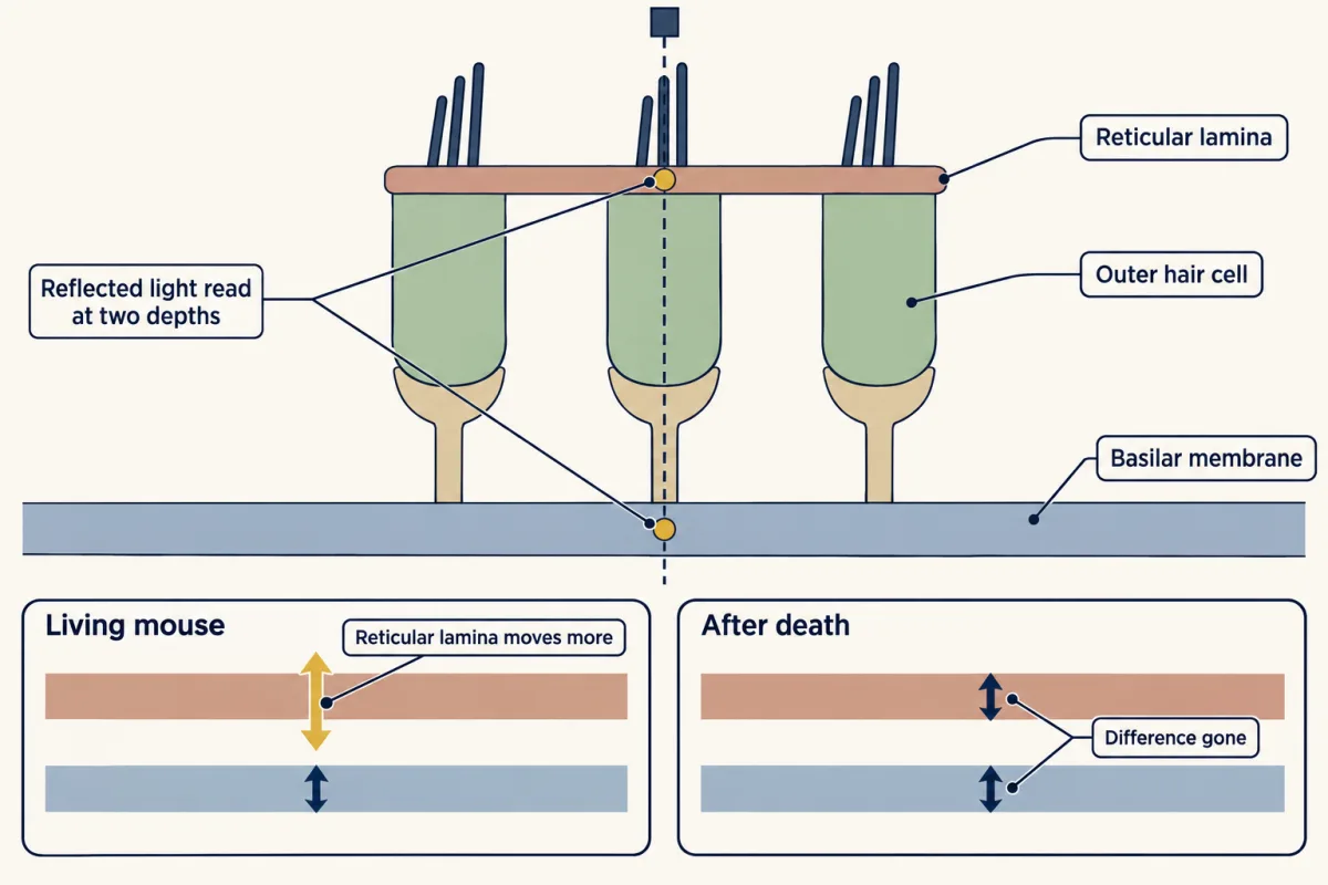
Older measurements mostly read the basilar membrane alone, at one place; newer optical methods read several depths in the living organ of Corti. Three terms help follow them.
- The reticular lamina is the top surface of the organ of Corti, where the hair bundles sit. The basilar membrane is its floor.
- In two-tone suppression, adding a second tone lowers the response to a probe tone, because the two interact through the cochlea’s nonlinearity wherever both excite outer hair cells. Changing the suppressor’s frequency shifts where along the cochlea its excitation peaks.
- The buildup distance is the length of cochlea, basal to the peak, over which the gain is gathered.
Ren and colleagues found larger reticular-lamina than basilar-membrane motion at a basal site in living mice at lower sound levels, and the differences in magnitude and phase disappeared postmortem. They read their data as showing that outer hair cells do not boost the basilar membrane by local feedback. Instead, they proposed, the cells drive the reticular lamina over a broad range of frequencies, and that motion acts on the travelling wave through the fluid. Lee and colleagues, imaging the apex, found radial tuning that persisted postmortem, which they took to suggest a passive contribution within the organ of Corti.
Dewey and colleagues tested the Ren idea with two-tone suppression. The inference needs two conditions. A suppressor that lowers the probe response while barely moving the measurement site points to gain contributed from where it acts, provided it is shown to reduce outer hair cell force there. And suppression confined to nearby suppressors supports a limited buildup only if the distant ones were effective in the regions tested. Varying suppressor level, and measuring each suppressor’s own excitation as well as the probe response, checks both. They concluded that forces from outer hair cells accumulate mainly near the peak of the travelling wave, and found that reticular-lamina gain, like basilar-membrane gain, builds up only near the peak. They wrote that this contradicts a global role for reticular-lamina motion. The studies used different sites, questions and readouts, but they also disagree. The unsettled point is how far along the cochlea gain is built, and how much is local.
Design problem
Two groups measure motion inside the living cochlea (Ren and colleagues, and Dewey and colleagues). One favours gain that accumulates along the cochlea; the other favours gain made locally. Design an experiment to separate them, then interpret this result: in a living mouse, reticular-lamina motion exceeds basilar-membrane motion at and below the best frequency, and the difference disappears postmortem.
Saved in this browser only.
One way to do it
Measure motion at matched sites with depth and direction resolved, so the reticular lamina and the basilar membrane are read in the same radial segment. Probe near the best frequency, then add suppressing tones whose excitation peaks lie at chosen distances basal to the site, each at several levels. Record each suppressor’s own motion at the site, check that it acts in the region it targets, and apply the two conditions above. Repeat each condition postmortem in the same animal as a control.
Dewey and colleagues made the suppression measurements in living mice at an apical site with a 60 dB SPL probe near the best frequency; they did not repeat them after death, so the postmortem control is an extension proposed here. They estimated buildup distances of 0.95 +/- 0.024 mm (mean +/- SEM, n = 8) for the basilar membrane and 0.71 +/- 0.042 mm (n = 10) for the reticular lamina. That points to a limited stretch of cochlea contributing, not the whole base.
For the stated result: a difference that vanishes after death depends on the living state, and larger reticular-lamina motion shows the organ of Corti is not moving as one block. The result does not show where the energy comes from or how it is split between bundles and cell bodies. Motion is not work done. One basal site in one strain is not a map of the cochlea, and the basal site of Ren and the apical site of Dewey cannot be assumed to behave alike.
Going deeper
The prestin structures, study by study
- Ge and colleagues (Cell, 2021) solved full-length human prestin, expressed in HEK293 GnTI-minus cells and purified into detergent micelles or lipid nanodiscs. An ordered ring of lipid surrounds the protein. The authors assigned the chloride structure to a contracted state and the salicylate structure to an expanded state.
- Bavi and colleagues (Nature, 2021) resolved recombinant dolphin prestin in six distinct states and interpreted salicylate inhibition as the protein being held in one conformation.
- Butan and colleagues (Nature Communications, 2022) solved gerbil prestin at 3.6 angstroms. Each protomer has 14 transmembrane helices, and the cytoplasmic STAS domains are swapped. The S398E result also shows why controls matter: before reading drug insensitivity of NLC as evidence against a chloride-only extrinsic voltage sensor, you need expression, localization and baseline NLC for each mutant.
A later study combined molecular dynamics of human prestin with fluorescence and functional tests on rat prestin constructs (in cultured CHO cells and Xenopus oocytes) and supported an elevator-like movement of a transport domain, while stating that chloride’s role was still unclear (Kuwabara and colleagues, Nature Communications, 2023).
Efferent feedback: turning the gain down
Medial olivocochlear efferents release acetylcholine, which acts through nicotinic receptors containing the alpha-9 and alpha-10 subunits. Calcium entry activates nearby calcium-dependent potassium channels. By shunting and hyperpolarizing the cell, acetylcholine shrinks the voltage swing that drives prestin, which reduces the cell’s electromotile response and so turns down the amplifier’s gain (reviewed by Fuchs and Lauer, 2019).
In mice with altered efferent receptors, the same noise exposure had different outcomes. Boero and colleagues (2018) exposed animals at postnatal day 21 to 1 to 16 kHz noise at 100 dB SPL for one hour. Wild-type mice recovered thresholds but lost ribbon synapses. Mice lacking Chrna9 kept permanent threshold elevations, and mice with a gain-of-function receptor (L9’T) resisted the same protocol. That is conditional protection in constitutive mouse genotypes at one age and one exposure, not a treatment and not evidence about people. The same study recorded the 2f1 - f2 distortion product in these mice.
Three optical studies, in detail
- Ren, He and Kemp (PNAS, 2016) used anaesthetized CBA/CaJ mice aged 3 to 5 weeks, at a basal site about 0.85 mm from the base. Reticular-lamina motion exceeded basilar-membrane motion at lower frequencies and near the best frequency at 20 to 50 dB SPL, but not significantly at 60 to 80 dB SPL.
- Lee and colleagues (J. Neurosci., 2016) imaged the apex through the intact otic capsule in mice aged P28 to P42, with tones from 2 to 13 kHz.
- Dewey, Applegate and Oghalai (J. Neurosci., 2019) used 4 to 6 week old CBA/CaJ mice and a site whose best frequency was about 9 to 9.5 kHz, with two-tone suppression.
Your notes
Select any text in the lesson to highlight it or add a note to it. Your highlights and notes are saved in this browser and collected in your notebook.
This browser is not letting the site save anything (a private window or strict privacy settings), so highlights and notes will be lost when you leave the page.
How we measure it
Single-particle cryo-EM
Purified protein is frozen in a thin film and imaged, and many particle images are averaged into a three-dimensional map. It shows the architecture and ligand-associated states of the protein, but it does not measure force, work or voltage-driven movement.
Whole-cell voltage clamp with nonlinear-capacitance analysis
The voltage of a cell is stepped or ramped while capacitance is measured. A bell-shaped capacitance peak reports voltage-dependent displacement of charge, and a two-state Boltzmann fit gives a half-activation voltage and an effective charge.
Optical coherence vibrometry with two-tone suppression
Light reflected from several depths of the living cochlea gives motion of the basilar membrane and the reticular lamina at once. A second, suppressing tone then tests which regions of the cochlea set the gain at the measured site.
Ear-canal acoustic recording with signal averaging
A microphone in the sealed ear canal records the response to clicks or to two pure tones, and averaging separates the faint cochlear emission from noise. It tests outer hair cell function without entering the ear.
Practice questions on this lesson (3) → MCAT-style, original, each with an explanation
Where this lesson fits
Before thisReview first
- Five Ways to Turn a Stimulus into a CurrentThis course · Lesson 1
You need the hair-cell current and how a bent bundle opens channels from there, since the amplifier chain starts at bundle bending.
- The Hair Cell's Transduction ChannelThis course · Lesson 22
The channel's saturating current is the fast nonlinearity that makes the distortion product, and its current drives prestin.
After thisStudy next
- Hidden Hearing Loss, Gene Therapy and RegenerationThis course · Lesson 24
It takes the vulnerable outer hair cell gain further, to hidden loss after noise and to repair.
- Balance: Two Codes for Every Head MovementThis course · Lesson 25
It uses hair-cell transduction in balance organs, where no outer hair cell amplifier is involved.
Elsewhere on the siteFilms, simulations and method films in other courses
- The permeability cliffSimulation · Biochemistry
Prestin's charge-moving two-state behaviour rests on how a membrane's electric field acts on proteins in the bilayer.
Suggested by an AI model from the lessons themselves, then checked. How we use AI
Finish line
Test yourself
9 questions
Practice and MCAT-style, with explained answers.
Next · Lesson 24
Hidden Hearing Loss, Gene Therapy and Regeneration
A mouse can pass its hearing test after loud noise and still have lost about half the ribbon synapses at one place in the cochlea. What does a normal threshold actually tell you?
Continue →