Cell Signaling · Unit 1: How a cell knows anything
Binding: Affinity, Occupancy and Dose–Response
Rewritten on : new text and flashcards. Your notes and highlights stay, but the text around them may have moved.
Naloxone reverses a morphine overdose without reacting with morphine at all. What are the two drugs competing for?
Pause when the reading reaches a film, and offer to play it. Saved on this device.
Watch the film now, or keep listening
Builds on:Enzyme Kinetics: The Michaelis–Menten ModelProtein Binding and Allostery: How Hemoglobin Loads and Delivers OxygenWhy these?
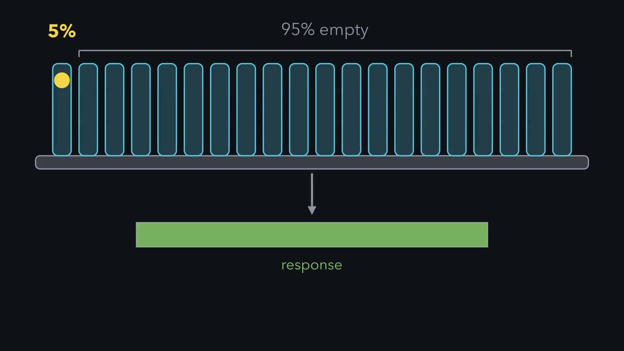 ▶ Watch A Full Response, Mostly Empty Receptors · 2:49
Read the transcript of “A Full Response, Mostly Empty Receptors”
Film transcript: A Full Response, Mostly Empty Receptors
This tissue is responding at its maximum. Yet only about five percent of its receptors are occupied. The other ninety-five percent are empty. How can a tissue give a full response with almost all of its receptors empty? To see why, start with binding. A ligand is any molecule that binds the receptor. The fraction of receptors occupied is the ligand concentration, divided by Kd plus the ligand concentration. Kd is the dissociation constant, the ligand concentration that fills half of the receptors. 5% occupancy comes at a ligand concentration far below Kd. Alfred Clark assumed that response is proportional to occupancy. The EC50 is the concentration that gives half of the maximum response.
With that assumption, the EC50 would equal Kd. But in 1956, Mark Nickerson reported that a tissue can reach its full response before all of its receptors are occupied. The reason is amplification in the pathway after the receptor. Picture a bottling line where the capper is the bottleneck. Once it runs at full speed, extra filling machines add nothing. Likewise, once enough receptors are occupied to saturate the slowest step downstream, more occupied receptors change nothing. The receptors that are not needed are called spare receptors. Together they make up the receptor reserve. Kd is a property of the drug and its receptor. The EC50 is a property of the whole pathway.
Say the pathway reaches its ceiling at 5% occupancy, and responds in proportion below that. Half of the maximum then needs only 2.5% occupancy. That puts the EC50 39 times below Kd, with no change in binding. You can prove a reserve by taking receptors away with an irreversible blocker. Remove half, and the curve moves right; remove 90%, and it moves further right. In this tissue, only when more than 95% are gone does the maximum fall. A real tissue has no sharp threshold, so the maximum sags gradually, but the order holds: shift first, fall later. Keep the rule: a full response does not mean every receptor is occupied.
Naloxone can pull a person out of a morphine overdose within minutes, and it never reacts with a single molecule of morphine. The two drugs compete for the same place on the same cells. This lesson asks how much of that place a given dose fills, how filling it becomes a response, and how two response curves can measure a drug’s grip on a receptor nobody has isolated.
A drug acts at a site it has to occupy
In 1905 John Langley, in Cambridge, tested two drugs on skeletal muscle. Nicotine made the muscle contract and curare prevented it, and both still worked after the nerve to the muscle had been cut and had degenerated. So the drugs were acting on the muscle itself. Langley called the thing they acted on the receptive substance. The shorter word, receptor, came from Paul Ehrlich, who had coined it a few years earlier while working on antitoxins, for toxins and nutrients rather than drugs.
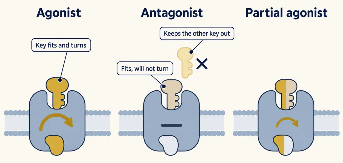
An agonist binds a receptor and switches it on. An antagonist binds the same receptor, does nothing there, and keeps the agonist out. In Emil Fischer’s lock-and-key picture, both keys fit and only the agonist turns. Some receptors are partly active with nothing bound, and some blockers, called inverse agonists, turn that background activity down.
The one idea to carry through this lesson. In the equilibrium, single-receptor model used here, the tissue sees the agonist’s occupancy. For one agonist acting on one unchanged receptor population in one tissue, the response is treated as a monotonic function of the fraction of receptors that agonist occupies. Binding sets that fraction, with Kd the only drug number in it; the agonist’s efficacy and the tissue’s amplifier turn it into a response that rises and then saturates, in a shape you usually do not know. Two results follow. Half-maximal effective concentration (EC50) is Kd seen through the agonist’s efficacy and the tissue’s amplifier. Equal responses on the monotonic, submaximal part of a curve mean equal occupancy (at the ceiling many occupancies give the same response), so when you compare two curves for the same agonist in one tissue below the maximum, the amplifier cancels, and the shift a competitive blocker causes measures the blocker’s own affinity. Each term is built below; come back to this box at the end.
Occupancy follows mass action
Picture a room with a fixed number of coat hooks. Coats go in, catch on hooks and drop off again. The hooks are receptors (R). The coats are ligand (L), any molecule that binds the receptor. The fraction of hooks holding a coat is the fractional occupancy.
The real mechanism is a reversible reaction, L + R ⇌ LR. Binding runs at a rate kon[L][R] and release at koff[LR]; at equilibrium the two are equal. The ratio of the rate constants is the dissociation constant, Kd = koff/kon, which also equals [L][R]/[LR]. Add the fact that every receptor is either empty or occupied, and you get the lesson’s binding equation:
In words The fraction of receptors occupied equals the ligand concentration divided by the dissociation constant plus the ligand concentration.
- [L]“L”
- the free ligand concentration, in solution and not bound. When there are far fewer receptors than ligand molecules, it is close to the concentration you added.nM
- Kd“K d”
- the dissociation constant, koff / kon: the free ligand concentration that occupies half of the receptorsnM
Sanity check At [L] = Kd, occupancy is Kd / 2Kd = 1/2. Far above Kd, occupancy approaches 1 but never reaches it.
Try one number
A ligand at three times its Kd: occupancy = 3Kd / (Kd + 3Kd) = 3/4.
Where it comes from optional
Step 1, equilibrium: kon[L][R] = koff[LR], so Kd = koff / kon = [L][R] / [LR].
Step 2, every receptor is empty (R) or occupied (LR): occupancy = [LR] / ([R] + [LR]).
Step 3, divide the top and bottom by [LR], and use [R]/[LR] = Kd/[L] from step 1: occupancy = 1 / (Kd/[L] + 1) = [L] / (Kd + [L]).
Need a refresher? reading an equation · log scales
So Kd, the free ligand concentration that half-fills the receptors, measures affinity: a small Kd means a tight grip. This is the same hyperbola as the Michaelis–Menten equation from the enzyme kinetics lesson, with occupancy in place of v/Vmax and Kd in place of Km, for the same reason: a fixed number of sites is being filled. One caution: Km combines several rate constants, while Kd is a pure binding constant.
Predict. What fraction of the receptors is occupied at [L] = Kd/9, and at [L] = 9 × Kd? How many times more ligand separates the two?
Check your prediction
At Kd/9, occupancy = (1/9) / (1 + 1/9) = 10%. At 9 × Kd, it is 9/(1 + 9) = 90%. Getting from 10% to 90% takes an 81-fold increase in ligand, nearly two powers of ten.
That is why these curves are drawn with concentration on a logarithmic axis. On a linear axis the low-dose end is crushed against the origin. On a log axis the hyperbola becomes a symmetric S-shaped curve with Kd at its midpoint. Try it in the explorer below.
- Apparent EC₅₀ (relative units)
- 1.0
- Ceiling response
- 100%
The dose that gives half-maximal response is the EC₅₀ — the lower it is, the more potent the drug. Efficacy is how high the curve can reach.
Potency (EC₅₀, the curve's horizontal position) and efficacy (Emax, its height) are independent. A competitive antagonist slides the curve right but can be overcome with more agonist; it never lowers the ceiling.
A binding curve that climbs from 10% to 90% in much less than 81-fold means the sites are not acting independently. That is cooperativity (see the lesson on protein binding and allostery). The rule is for binding curves: steps after the receptor can steepen a response curve, so a steep one says nothing about receptor cooperativity by itself.
Measuring occupancy directly
For most of the century after Langley, pharmacologists inferred receptors from responses. Direct binding measurements began in the 1960s with radioactive atropine on gut muscle, and by the early 1970s they had reached the nicotinic receptor and hormone receptors such as insulin’s.
In 1973 Candace Pert and Solomon Snyder at Johns Hopkins measured binding to the opiate receptor, as did two other groups the same year. They mixed radioactive naloxone with ground-up brain tissue, pulled the mixture through a filter, washed the filter and counted the radioactivity that stayed behind.
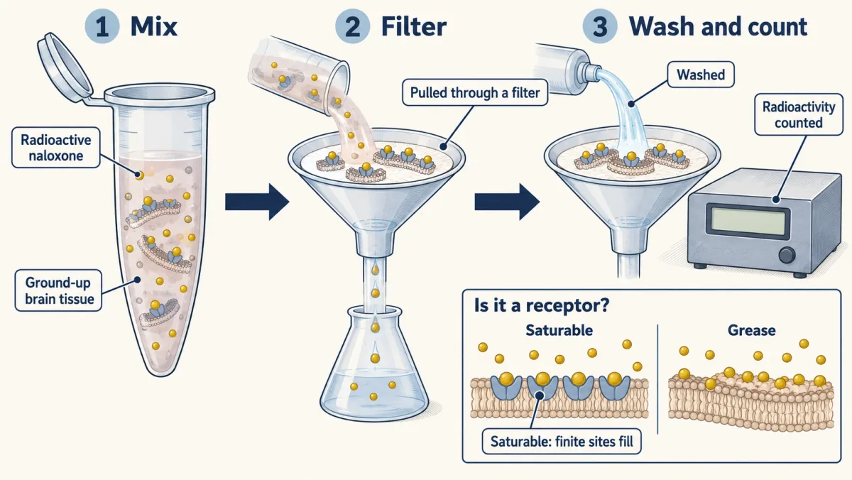
Brain is greasy and holds on to almost any small molecule. How do you show that what stuck is a receptor?
The binding has to be saturable. A finite set of sites fills up along the occupancy curve, while sticking to grease keeps rising with concentration. To see the saturable part, measure total binding, then measure it again with a large excess of unlabelled drug, which keeps the label off the specific sites and leaves only the nonspecific sticking. Total minus nonspecific is specific binding, the curve that saturates.
It has to be specific: unlabelled opiates pushed the radioactive naloxone off in the order of their known potency as drugs. And it has to be stereospecific. Levorphanol, an active opiate, displaced the label. Dextrorphan, its mirror image, has almost no opiate action and was far weaker. Grease cannot tell a molecule from its mirror image. A shaped pocket can.
The saturation curve hands you the numbers in the occupancy equation, measured on the site itself: a Kd, and the total count of sites, called Bmax. Langley’s receptive substance had become something you could count.
Response is not occupancy
Occupancy counts the receptors that have ligand bound. Response is what the tissue does: a muscle shortens, a gland secretes. A dose–response curve plots the response and has two numbers of its own. Half-maximal effective concentration (EC50) is the concentration that gives half of the drug’s maximum response; it measures potency: the lower the EC50, the less drug you need. Emax is the largest response the drug can produce, however much you add.
Four quantities lie behind those two numbers. Two belong to the drug at the receptor: affinity (Kd) and efficacy, how well the bound drug switches the receptor on. Two belong to the tissue: the number of receptors and the amplifier. EC50 mixes all four, which is why one agonist’s potency can differ between tissues. Emax shows efficacy only below the tissue’s ceiling: two full agonists with different efficacies can both reach the ceiling, and their difference then shows up in how far each EC50 sits below its Kd, or after receptors are removed.
A full agonist can drive the tissue to its maximum. A partial agonist levels off below it even when it occupies every receptor, like a key that turns the lock only part of the way. Whether a drug looks full or partial depends on the tissue too: in a tissue with many receptors, a weak key can still reach the maximum.
So a drug with an EC50 of 100 nM that reaches 100% is 100-fold less potent than one with an EC50 of 1 nM, with the same maximum; a drug with an EC50 of 1 nM that tops out at 40% is as potent, and less efficacious.
Predict. A tissue is responding fully to a full agonist. You add a partial agonist that acts at the same receptor. Does the response rise, stay or fall?
Check your prediction
It falls. Each receptor the weak key takes is one the strong key has lost, so the partial agonist behaves as an antagonist and pulls the response toward its own ceiling. It gets close to that ceiling only when it is concentrated enough to win most of the receptors.
The gap between the curves: receptor reserve
In 1926 Alfred Clark fitted the occupancy hyperbola, which A. V. Hill had used for nicotine in 1909 and Irving Langmuir for gas sticking to a surface, to the response of frog heart muscle to acetylcholine. He assumed that response is proportional to occupancy, which would make half-maximal effective concentration (EC50) equal to Kd. In 1956 Mark Nickerson published a short paper in Nature called “Receptor occupancy and tissue response.” He reported that a tissue can reach its full response before all of its receptors are occupied.
The reason is amplification after the receptor. Picture a bottling line where the capper is the bottleneck: once it runs at full speed, extra filling machines add nothing. Likewise, once enough receptors are occupied to saturate the slowest step downstream, more occupied receptors change nothing you can measure. This is the sharp version of an amplifier: proportional below the ceiling, flat at it. The receptors not needed are spare receptors, together the receptor reserve. They are ordinary receptors; the tissue has more copies than the pathway can use at once.
How far apart can EC50 and Kd be? Call p the fraction of receptors occupied when the response is half its maximum. At the EC50 the occupancy equation has to give p. Rearranged:
In words The EC50 equals the dissociation constant times p over one minus p, where p is the fraction of receptors occupied at half the maximum response.
- EC50“E C fifty”
- the agonist concentration that gives half of its maximum responsenM
- Kd“K d”
- the agonist's dissociation constant for the receptornM
- p“p”
- the fraction of receptors occupied when the response is half its maximum (between 0 and 1)
Sanity check If response is proportional to occupancy, p = 1/2 and EC50 = Kd, Clark's assumption. The smaller p, the further EC50 sits below Kd. The amplifier's shape appears only through p.
Try one number
Say the pathway reaches its ceiling at 5% occupancy and responds in proportion below that. Half the maximum needs 2.5% occupancy, so p = 0.025.
p / (1 − p) = 0.025 / 0.975 = 1/39. So EC50 = Kd/39, with no change in binding. One drug with a Kd of 100 nM has an EC50 of 100 nM where response tracks occupancy, and about 2.6 nM here.
Where it comes from optional
At the EC50, EC50 / (Kd + EC50) = p. Multiply out: EC50 = p × Kd + p × EC50. Collect terms: EC50 × (1 − p) = p × Kd.
Need a refresher? rates and “per”
Predict. A radioligand assay gives an agonist a Kd of 100 nM; in the intact cells its EC50 is 5 nM. What fraction of the receptors is occupied at half the maximum response? Does an EC50 below Kd prove a receptor reserve?
Check your prediction
About 4.8%: 5 / (100 + 5). But an EC50 below Kd is not proof by itself. A saturating, hyperbolic-type amplifier works on every agonist and puts its EC50 below its Kd, even for a partial agonist with no spare receptors (example in Going deeper). A reserve is present when the tissue reaches its full maximum with less than full receptor occupancy; an EC50 below Kd for an agonist that reaches that ceiling is evidence for it, and the receptor-inactivation experiment below tests it.
A common alternative to the sharp ceiling is a smooth amplifier. Give a smooth one the same EC50, Kd/39, and it agrees with the sharp one there and at the two ends but not in between: 5% occupancy gives about two thirds of the maximum, and 90% of the maximum needs about 19% occupancy. The film and the design problem below use the sharp picture; with the smooth one the maximum falls earlier (numbers in Going deeper).
Treating an EC50 as a binding affinity is a common error in the research literature. The gap is also a tool. If a treatment changes a drug’s EC50 and leaves its Kd alone, either the number of receptors or something after binding has changed, and you can look for it.
Design problem
A drug gives a full response when only about 5% of its receptors are occupied. State what that tells you, then design an experiment that would prove it.
Saved in this browser only.
One way to do it
What it tells you: for this drug in this tissue, about 95% of the receptors are spare. The reserve belongs to the pair of drug and tissue. A weaker agonist on the same tissue might need every receptor.
The experiment: take receptors away and watch the curve. Use an irreversible antagonist, a blocker that bonds covalently to the receptor and cannot be washed off or outcompeted. Treat strips of tissue so that different fractions of the receptors are destroyed, wash, then run a full agonist dose–response curve on each strip. In matched samples, count with a radioactive ligand what fraction of the receptors each treatment removed.
The predictions, in the sharp-ceiling picture and taking the 5% figure at face value:
- Half of the receptors gone. The 5% of the original total it needs is now 10% of the survivors. You still get a full response at a higher dose, so the curve moves right.
- 90% gone. That 5% is now half of the survivors. Still a full response, further right.
- More than 95% gone. Even with every survivor occupied, the tissue is short of the number it needs. Now the maximum falls.
A rightward shift first and a lower maximum afterwards is the proof. With no reserve, the maximum would start to fall with the first receptors lost. Real tissues have no sharp threshold, so the maximum sags earlier and more gradually, but the order of events is the same.
As a control, a second agonist acting through a different receptor should keep its full maximum, which shows that the blocker left the downstream pathway undamaged.
Blocking the receptor: the shape of the shift names the blocker
Go back to the coat hooks and throw in decoy coats. They take up hooks and produce nothing.
A competitive antagonist binds reversibly at the agonist’s own site. A receptor can hold the agonist or the antagonist, never both. Add enough agonist and it wins the hooks back, so the maximum is unchanged. What changes is the dose you need: on a log axis the whole curve slides right, parallel to itself. Naloxone does this to morphine. The size of the slide is the dose ratio: the agonist concentration needed for a given response with the antagonist present, divided by the concentration needed without it.
Predict. You work on a tissue you know almost nothing about: not how many receptors it has, how much reserve, or how many steps lie between receptor and contraction. You measure the agonist’s dose–response curve with and without the antagonist. Can those two curves tell you how tightly the antagonist binds?
Check your prediction
Yes. Pick a response level, say 30% of the maximum: without the antagonist the agonist needs concentration A to give it, with the antagonist A′. In the scoped model above, equal responses on the monotonic, submaximal part of the curve mean equal agonist occupancy, so the amplifier cancels and only binding is left.
Write the agonist’s occupancy without and with the antagonist (whose share of the receptors adds [B]/KB to the bottom of the fraction), set the two equal, and solve:
In words The dose ratio equals one plus the antagonist concentration divided by the antagonist's own dissociation constant.
- A, A′“A and A prime”
- agonist concentrations giving the same response without and with the antagonistnM
- [B]“B”
- the free antagonist concentrationnM
- KB“K B”
- the antagonist's dissociation constant for the receptor: the concentration that would occupy half the receptors if it were alonenM
Sanity check With no antagonist, the dose ratio is 1. At [B] = KB it is 2; at [B] = 10 × KB it is 11. The agonist's Kd, its efficacy, the receptor number and the amplifier do not appear.
Try one number
An agonist’s EC50 of 10 nM moves to 110 nM with 100 nM of antagonist, same maximum. Dose ratio 11, so [B]/KB = 10 and KB = 10 nM.
Then 1000 nM of antagonist should give a dose ratio of 101, an EC50 of 1010 nM. If it does, simple competition holds.
Where it comes from optional
Step 1, equal submaximal response means equal occupancy, where KA is the agonist’s dissociation constant: (A/KA) / (1 + A/KA) = (A′/KA) / (1 + A′/KA + [B]/KB).
Step 2, cross-multiply: A × (1 + A′/KA + [B]/KB) = A′ × (1 + A/KA).
Step 3, expand: the A × A′/KA terms on both sides cancel, leaving A × (1 + [B]/KB) = A′.
Need a refresher? rates and “per” · log scales
So an antagonist at ten times its KB moves every agonist’s curve for that receptor elevenfold, in every tissue that carries it, as long as the assumptions at the end of the lesson hold. That is why antagonist affinities became the fingerprints that told one receptor type from another, long before any receptor was isolated.
Schild’s test: is it really competition?
J. H. Gaddum wrote down the competition equation in 1937. Heinz Schild turned it into a measurement in 1947 and, with Arunlakshana in 1959, into a test. Take logs of the rearranged equation:
log(dose ratio − 1) = log [B] − log KB
Plot log(dose ratio − 1) against log [B] for several antagonist concentrations. Simple competition at equilibrium predicts a straight line of slope 1 that crosses zero at log KB. Schild’s pA2 is the negative log of the antagonist concentration that gives a dose ratio of 2. At that point [B] = KB, so pA2 equals −log KB, but only when the slope is 1, because only then does the competition equation hold at every [B].
A slope other than 1 means an assumption failed: the antagonist had not reached equilibrium, the tissue was removing the agonist, the antagonist bound elsewhere and changed the agonist’s affinity, or more than one receptor contributed. A plot that curves at high [B] signals the same, and a slope of 1 over a narrow range of [B] does not rule these out. The test tells you the simple reading is unsafe even when it cannot say which assumption broke.
Blockers that more agonist cannot overcome
Such blockers are called insurmountable; a competitive antagonist, which more agonist does overcome, is surmountable. A non-competitive antagonist binds somewhere else on the receptor, or acts after it, and stops the receptor from responding. An irreversible antagonist, the covalent blocker of the design problem, binds at the agonist’s own site. The signature of both is a lower maximum, but not always at once:
| Blocker | What happens to the agonist curve |
|---|---|
| Competitive antagonist | Parallel shift right, same maximum; Schild slope 1 |
| Irreversible (such as β-funaltrexamine) | With a reserve, shift right first, then the maximum falls; with none, the maximum falls from the start |
| Insurmountable allosteric | Varies with how the blocker changes the agonist’s affinity and efficacy |
| Non-competitive, acting after the receptor (such as a block of a step in the contraction itself) | Lower maximum; any shift depends on the step blocked |
| Partial agonist added with the full agonist | Response raised at low full-agonist doses by the partial agonist’s own effect; above the partial agonist’s ceiling, competition shifts the curve right, but enough full agonist still reaches the full maximum |
Potency orders as fingerprints
Agonist potency rankings sorted receptors into types too. Blood delivers adrenaline to every organ at much the same concentration, yet it narrows blood vessels in the skin and relaxes airways, so the difference lies in the tissues. In 1948 Raymond Ahlquist ranked six adrenaline-like drugs by potency on many tissues. One kind of pocket should give much the same order everywhere, he reasoned. For vasoconstriction, adrenaline and noradrenaline ranked high and isoproterenol low. For vasodilation, relaxation of the uterus and stimulation of the heart, the ranking ran nearly the other way. No third order appeared, so he proposed two kinds and named them alpha and beta.
Back to the opening question
Naloxone and morphine compete for the opiate receptor Pert’s assay counted. In a simple single-receptor preparation at equilibrium, naloxone takes receptors without switching them on and moves morphine’s concentration-response curve right by a dose ratio of 1 + [naloxone]/KB. This competition reduces the mu-opioid-receptor signalling that drives respiratory depression, but clinical reversal is time-dependent and is not predicted by that equilibrium ratio alone. Naloxone never touches a morphine molecule; it changes how many receptors morphine occupies. Buprenorphine, a partial agonist at the same receptor, has a maximum set by its efficacy and by each tissue’s receptor reserve, and against a full agonist it acts partly as a blocker.
Where the idea stops
The rule assumes equilibrium, one class of independent sites, a response that is monotonic with agonist occupancy below its ceiling, free concentrations close to those added (no depletion or uptake), no desensitization during the curve, an antagonist that acts only at the receptor with no efficacy of its own (neither a partial nor an inverse agonist), and unchanged receptor number.
- Across agonists. The amplifier’s input includes efficacy, so two agonists at equal response are not at equal occupancy. The rule compares one agonist with itself.
- Irreversible antagonists change receptor number, and so what the tissue does with a given occupancy. Furchgott’s method uses exactly this.
- Allosteric modulators, slow equilibration, uptake, more than one receptor. These can make a Schild plot curved or give it a non-unit slope, but a unit-slope plot does not exclude them.
- Pathway-selective (biased) agonists. The amplifier depends on which response you measure, so one efficacy value does not transfer.
Going deeper
A smooth amplifier: the operational model
In the operational model of Black and Leff (1983), response = Em × τ[A] / (KA + (1 + τ)[A]), where Em is the system maximum and τ is receptor density divided by the concentration of occupied receptor that gives half of Em. Then half-maximal effective concentration (EC50) = KA/(1 + τ) and the observed maximum is Em × τ/(1 + τ). With τ = 38, EC50 = KA/39 and occupancy at the EC50 is 2.5%, as with the sharp 5% ceiling: same p, same EC50, different amplifiers. Removing receptors lowers τ:
| Receptors left | Smooth (τ = 38): maximum as % of untreated, EC50 | Sharp ceiling at 5%: maximum, EC50 |
|---|---|---|
| 100% | 100%, KA/39 | 100%, Kd/39 |
| 50% | 97.5%, KA/20 | 100%, Kd/19 |
| 10% | 81%, KA/4.8 | 100%, Kd/3 |
| 5% | 67%, KA/2.9 | 100%, Kd |
| 2% | 44%, KA/1.8 | 40%, Kd |
EC50 moves toward KA before the maximum collapses, and Furchgott’s receptor-inactivation method (1966) uses that behaviour to estimate an agonist’s KA. The model also shows why EC50 below Kd is not proof of a reserve: a partial agonist with τ = 1 reaches half of Em and still has EC50 = KA/2.
Who named efficacy
Nickerson’s paper is the usual citation for spare receptors. The idea that response is not proportional to occupancy, and the term efficacy, are usually credited to Stephenson (1956), building on Ariëns’s “intrinsic activity” (1954).
Equilibrium constants in a living tissue
Concentrations in a living tissue can change faster than binding equilibrates, so the time a drug stays on its receptor, set by koff rather than Kd, may matter more than Kd. How far equilibrium constants predict effect in vivo is still argued over.
Your notes
Select any text in the lesson to highlight it or add a note to it. Your highlights and notes are saved in this browser and collected in your notebook.
This browser is not letting the site save anything (a private window or strict privacy settings), so highlights and notes will be lost when you leave the page.
How we measure it
Isolated-tissue bioassay (organ bath)
A strip of muscle or a piece of heart is kept alive in warm, oxygenated salt solution and connected to a recorder. You add a drug at rising concentrations and measure the contraction or relaxation at each one. The result is a dose-response curve, from which EC50 and Emax are read.
Radioligand binding assay
Membranes are incubated with a radioactive ligand, then filtered and washed, and the radioactivity left on the filter is counted. Repeating the incubation with a large excess of unlabelled ligand measures nonspecific sticking, which is subtracted. The specific binding that remains saturates, and its curve gives Kd and the number of sites (Bmax).
Schild analysis
You measure agonist dose-response curves at several concentrations of an antagonist and calculate the dose ratio for each. For a competitive antagonist, log(dose ratio − 1) plotted against log antagonist concentration is a straight line of slope 1. The point where the line crosses zero sits at log KB, which gives KB, the antagonist's dissociation constant.
Irreversible receptor inactivation
A tissue is treated with a blocker that bonds covalently to the receptor and is then washed, so that a fraction of the receptors is permanently removed. Comparing agonist curves before and after shows whether the curve moves right before its maximum falls. That order reveals a receptor reserve.
Practice questions on this lesson (3) → MCAT-style, original, each with an explanation
Where this lesson fits
Before thisReview first
- Enzyme Kinetics: The Michaelis–Menten ModelBiochemistry · College: going further
The occupancy hyperbola here is the same saturation curve as Michaelis–Menten, so you need Km and saturation from there.
- Protein Binding and Allostery: How Hemoglobin Loads and Delivers OxygenBiochemistry · College: going further
You need binding curves, Kd and cooperativity from there to read why steep curves signal interacting sites.
After thisStudy next
- A Field Guide to ReceptorsThis course · Lesson 4
It uses antagonist affinities and potency orders to tell receptor types apart, as Ahlquist did.
- GPCRs and Trimeric G ProteinsThis course · Lesson 12
It follows how an occupied receptor drives a G protein, the amplification step behind receptor reserve.
- Circuits: Amplification, Feedback, Adaptation and SwitchesThis course · Lesson 5
It takes the amplifier between occupancy and response further, with gain, feedback and switches.
Suggested by an AI model from the lessons themselves, then checked. How we use AI
Finish line
Test yourself
8 questions
Practice and MCAT-style, with explained answers.
Next · Lesson 4
A Field Guide to Receptors
Acetylcholine starts a muscle twitch and slows a heart. Same molecule: what decides what it means?
Continue →